- 1. OptaPlanner Introduction
- 2. Quick Start
- 3. Use Cases and Examples
- 4. Planner Configuration
- 5. Score Calculation
- 5.1. Score Terminology
- 5.2. Choose a Score Definition
- 5.3. Calculate the
Score - 5.4. Score Calculation Performance Tricks
- 5.4.1. Overview
- 5.4.2. Average Calculation Count Per Second
- 5.4.3. Incremental Score Calculation (with Delta's)
- 5.4.4. Avoid Calling Remote Services During Score Calculation
- 5.4.5. Pointless Constraints
- 5.4.6. Built-in Hard Constraint
- 5.4.7. Other Score Calculation Performance Tricks
- 5.4.8. Score Trap
- 5.4.9. stepLimit Benchmark
- 5.4.10. Fairness Score Constraints
- 5.5. Explaining the Score: Using Score Calculation Outside the
Solver
- 6. Optimization Algorithms
- 6.1. Search Space Size in the Real World
- 6.2. Does Planner Find the Optimal Solution?
- 6.3. Architecture Overview
- 6.4. Optimization Algorithms Overview
- 6.5. Which Optimization Algorithms Should I Use?
- 6.6. Power tweaking or default parameter values
- 6.7. Solver Phase
- 6.8. Scope Overview
- 6.9. Termination
- 6.10. SolverEventListener
- 6.11. Custom Solver Phase
- 7.
Moveand Neighborhood Selection - 7.1.
Moveand Neighborhood Introduction - 7.2. Generic MoveSelectors
- 7.3. Combining Multiple
MoveSelectors - 7.4. EntitySelector
- 7.5. ValueSelector
- 7.6. General
SelectorFeatures - 7.6.1.
CacheType: Create Moves Ahead of Time or Just In Time - 7.6.2. SelectionOrder: Original, Sorted, Random, Shuffled or Probabilistic
- 7.6.3. Recommended Combinations of
CacheTypeandSelectionOrder - 7.6.4. Filtered Selection
- 7.6.5. Sorted Selection
- 7.6.6. Probabilistic Selection
- 7.6.7. Limited Selection
- 7.6.8. Mimic Selection (Record/Replay)
- 7.6.9. Nearby Selection
- 7.6.1.
- 7.7. Custom Moves
- 7.1.
- 8. Exhaustive Search
- 9. Construction Heuristics
- 10. Local Search
- 11. Evolutionary Algorithms
- 12. Hyperheuristics
- 13. Partitioned Search
- 14. Benchmarking And Tweaking
- 14.1. Find The Best
SolverConfiguration - 14.2. Benchmark Configuration
- 14.2.1. Add Dependency On
optaplanner-benchmark - 14.2.2. Build And Run A
PlannerBenchmark - 14.2.3. SolutionFileIO: Input And Output Of Solution Files
- 14.2.4. Warming Up The HotSpot Compiler
- 14.2.5. Benchmark Blueprint: A Predefined Configuration
- 14.2.6. Write The Output Solution Of Benchmark Runs
- 14.2.7. Benchmark Logging
- 14.2.1. Add Dependency On
- 14.3. Benchmark Report
- 14.4. Summary Statistics
- 14.4.1. Best Score Summary (Graph And Table)
- 14.4.2. Best Score Scalability Summary (Graph)
- 14.4.3. Winning Score Difference Summary (Graph And Table)
- 14.4.4. Worst Score Difference Percentage (ROI) Summary (Graph and Table)
- 14.4.5. Average Calculation Count Summary (Graph and Table)
- 14.4.6. Time Spent Summary (Graph And Table)
- 14.4.7. Time Spent Scalability Summary (Graph)
- 14.4.8. Best Score Per Time Spent Summary (Graph)
- 14.5. Statistic Per Dataset (Graph And CSV)
- 14.5.1. Enable A Problem Statistic
- 14.5.2. Best Score Over Time Statistic (Graph And CSV)
- 14.5.3. Step Score Over Time Statistic (Graph And CSV)
- 14.5.4. Calculate Count Per Second Statistic (Graph And CSV)
- 14.5.5. Best Solution Mutation Over Time Statistic (Graph And CSV)
- 14.5.6. Move Count Per Step Statistic (Graph And CSV)
- 14.5.7. Memory Use Statistic (Graph And CSV)
- 14.6. Statistic Per Single Benchmark (Graph And CSV)
- 14.6.1. Enable A Single Statistic
- 14.6.2. Constraint Match Total Best Score Over Time Statistic (Graph And CSV)
- 14.6.3. Constraint Match Total Step Score Over Time Statistic (Graph And CSV)
- 14.6.4. Picked Move Type Best Score Diff Over Time Statistic (Graph And CSV)
- 14.6.5. Picked Move Type Step Score Diff Over Time Statistic (Graph And CSV)
- 14.7. Advanced Benchmarking
- 14.1. Find The Best
- 15. Repeated Planning
- 16. Integration
- 17. Development

OptaPlanner is a lightweight, embeddable constraint satisfaction engine which optimizes planning problems. It solves use cases such as:
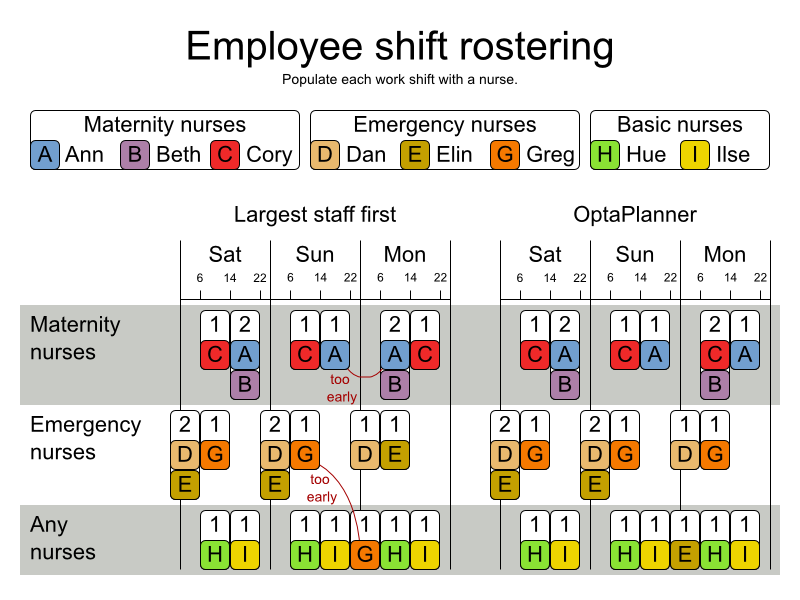
Employee shift rostering: timetabling nurses, repairmen, ...
Agenda scheduling: scheduling meetings, appointments, maintenance jobs, advertisements, ...
Educational timetabling: scheduling lessons, courses, exams, conference presentations, ...
Vehicle routing: planning vehicles (trucks, trains, boats, airplanes, ...) with freight and/or people
Bin packing: filling containers, trucks, ships and storage warehouses, but also cloud computers nodes, ...
Job shop scheduling: planning car assembly lines, machine queue planning, workforce task planning, ...
Cutting stock: minimizing waste while cutting paper, steel, carpet, ...
Sport scheduling: planning football leagues, baseball leagues, ...
Financial optimization: investment portfolio optimization, risk spreading, ...
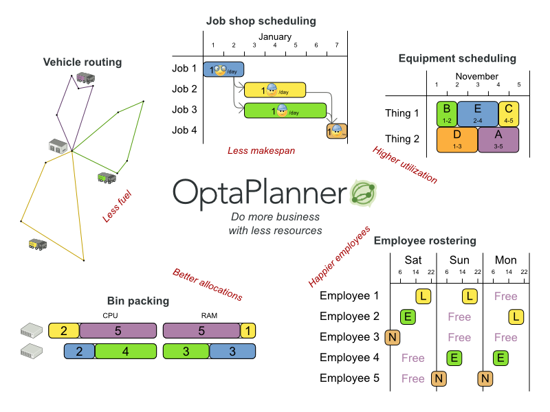
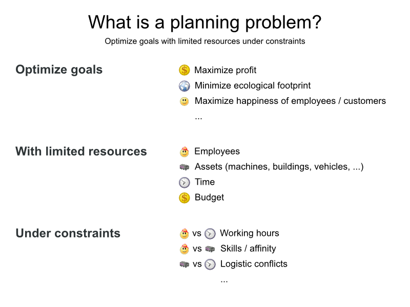
Every organization faces planning problems: provide products or services with a limited set of constrained resources (employees, assets, time and money). OptaPlanner optimizes such planning to do more business with less resources. This is known as Constraint Satisfaction Programming (which is part of the Operations Research discipline).
OptaPlanner helps normal JavaTM programmers solve constraint satisfaction problems efficiently. Under the hood, it combines optimization heuristics and metaheuristics with very efficient score calculation.
OptaPlanner is open source software, released under the Apache Software License 2.0. This license is very liberal and allows reuse for commercial purposes. Read the layman's explanation.
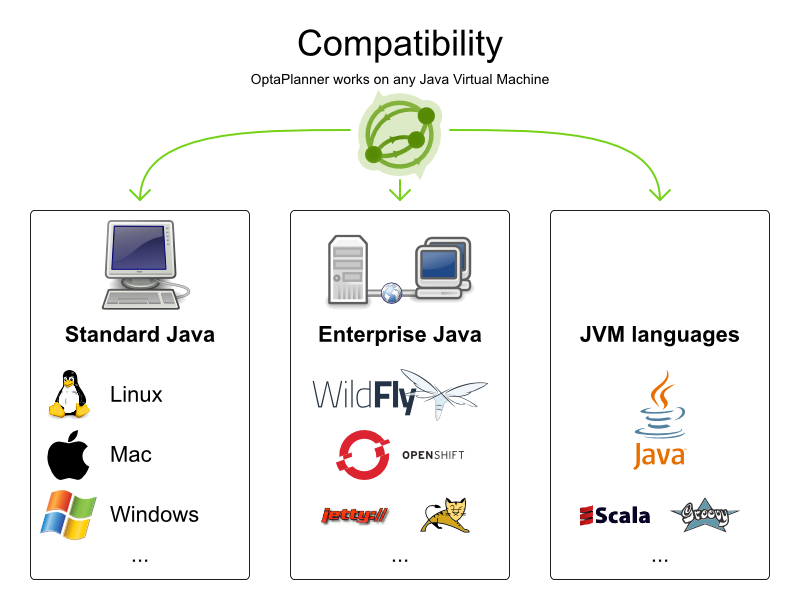
OptaPlanner is 100% pure JavaTM and runs on any JVM 1.6 or higher. It integrates very easily with other JavaTM technologies. OptaPlanner is available in the Maven Central Repository.
All the use cases above are probably NP-complete or harder. In layman's terms, NP-complete means:
It's easy to verify a given solution to a problem in reasonable time.
There is no silver bullet to find the optimal solution of a problem in reasonable time (*).
Note
(*) At least, none of the smartest computer scientists in the world have found such a silver bullet yet. But if they find one for 1 NP-complete problem, it will work for every NP-complete problem.
In fact, there's a $ 1,000,000 reward for anyone that proves if such a silver bullet actually exists or not.
The implication of this is pretty dire: solving your problem is probably harder than you anticipated, because the 2 common techniques won't suffice:
A Brute Force algorithm (even a smarter variant) will take too long.
A quick algorithm, for example in bin packing, putting in the largest items first, will return a solution that is far from optimal.
By using advanced optimization algorithms, OptaPlanner does find a good solution in reasonable time for such planning problems.
Usually, a planning problem has at least 2 levels of constraints:
A (negative) hard constraint must not be broken. For example: 1 teacher can not teach 2 different lessons at the same time.
A (negative) soft constraint should not be broken if it can be avoided. For example: Teacher A does not like to teach on Friday afternoon.
Some problems have positive constraints too:
A positive soft constraint (or reward) should be fulfilled if possible. For example: Teacher B likes to teach on Monday morning.
Some basic problems (such as N Queens) only have hard constraints. Some problems have 3 or more levels of constraints, for example hard, medium and soft constraints.
These constraints define the score calculation (AKA fitness function) of a planning problem. Each solution of a planning problem can be graded with a score. With OptaPlanner, score constraints are written in an Object Oriented language, such as Java code or Drools rules. Such code is easy, flexible and scalable.
A planning problem has a number of solutions. There are several categories of solutions:
A possible solution is any solution, whether or not it breaks any number of constraints. Planning problems tend to have an incredibly large number of possible solutions. Many of those solutions are worthless.
A feasible solution is a solution that does not break any (negative) hard constraints. The number of feasible solutions tends to be relative to the number of possible solutions. Sometimes there are no feasible solutions. Every feasible solution is a possible solution.
An optimal solution is a solution with the highest score. Planning problems tend to have 1 or a few optimal solutions. There is always at least 1 optimal solution, even in the case that there are no feasible solutions and the optimal solution isn't feasible.
The best solution found is the solution with the highest score found by an implementation in a given amount of time. The best solution found is likely to be feasible and, given enough time, it's an optimal solution.
Counterintuitively, the number of possible solutions is huge (if calculated correctly), even with a small dataset. As you can see in the examples, most instances have a lot more possible solutions than the minimal number of atoms in the known universe (10^80). Because there is no silver bullet to find the optimal solution, any implementation is forced to evaluate at least a subset of all those possible solutions.
OptaPlanner supports several optimization algorithms to efficiently wade through that incredibly large number of possible solutions. Depending on the use case, some optimization algorithms perform better than others, but it's impossible to tell in advance. With OptaPlanner, it is easy to switch the optimization algorithm, by changing the solver configuration in a few lines of XML or code.
To try it now:
Download a release zip of OptaPlanner from the OptaPlanner website and unzip it.
Open the directory
examplesand run the script.Linux or Mac:
$ cd examples
$ ./runExamples.sh
Windows:
$ cd examples
$ runExamples.bat
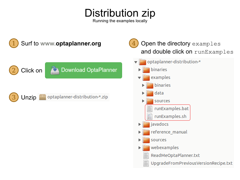
The Examples GUI application will open. Pick an example to try it out:
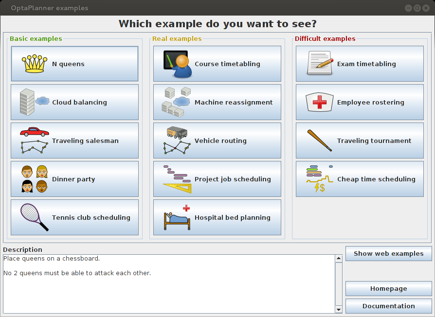
Note
OptaPlanner itself has no GUI dependencies. It runs just as well on a server or a mobile JVM as it does on the desktop.
Besides the GUI examples, there are also a set of webexamples to try out:
Download a JEE application server, such as JBoss EAP or WildFly and unzip it.
Download a release zip of OptaPlanner from the OptaPlanner website and unzip it.
Open the directory
webexamplesand deploy theoptaplanner-webexamples-*.warfile on the JEE application server.Surf to http://localhost:8080/optaplanner-webexamples-*/ (replace the
*with the actual version).
Note
The webexamples (but not OptaPlanner itself) require several JEE API's (such as Servlet, JAX-RS and CDI)
to run. To successfully deploy optaplanner-webexamples-*.war on a servlet container (such as
Jetty or Tomcat), instead of on a real JEE application server (such as WildFly), add the missing implementation
libraries (for example RestEasy and Weld) in the war manually.
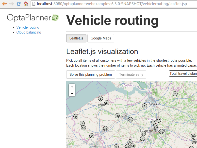
Pick an example to try it out, such as the Vehicle Routing example:
To run the examples in your favorite IDE:
Configure your IDE:
In IntelliJ IDEA, NetBeans or a non-vanilla Eclipse, just open the file
examples/sources/pom.xmlas a new project, the maven integration will take care of the rest.In a vanilla Eclipse (which lacks the M2Eclipse plugin), open a new project for the directory
examples/sources.Add all the jars to the classpath from the directory
binariesand the directoryexamples/binaries, except for the fileexamples/binaries/optaplanner-examples-*.jar.Add the Java source directory
src/main/javaand the Java resources directorysrc/main/resources.
Create a run configuration:
Main class:
org.optaplanner.examples.app.OptaPlannerExamplesAppVM parameters (optional):
-Xmx512M -server
Run that run configuration.
To run a specific example directly and skip the example selection window, run its App
class (for example CloudBalancingApp) instead of
OptaPlannerExamplesApp.
The OptaPlanner jars are also available in the central maven repository (and also in the JBoss maven repository).
If you use Maven, add a dependency to optaplanner-core in your project's
pom.xml:
    <dependency>
      <groupId>org.optaplanner</groupId>
      <artifactId>optaplanner-core</artifactId>
    </dependency>
This is similar for Gradle, Ivy and Buildr. To identify the latest version, check the central maven repository.
Because you might end up using other OptaPlanner modules too, it's recommended to import the
optaplanner-bom in Maven's dependencyManagement so the OptaPlanner version
is specified only once:
  <dependencyManagement>
    <dependencies>
      <dependency>
        <groupId>org.optaplanner</groupId>
        <artifactId>optaplanner-bom</artifactId>
        <type>pom</type>
        <version>...</version>
        <scope>import</scope>
      </dependency>
      ...
    </dependencies>
  </dependencyManagement>
If you're still using ANT (without Ivy), copy all the jars from the download zip's
binaries directory in your classpath.
Note
The download zip's binaries directory contains far more jars then
optaplanner-core actually uses. It also contains the jars used by other modules, such as
optaplanner-benchmark.
Check the maven repository pom.xml files to determine the minimal dependency set of a
specific module (for a specific version).
It's easy to build OptaPlanner from source:
Set up Git and clone
optaplannerfrom GitHub (or alternatively, download the zipball):$ git clone git@github.com:droolsjbpm/optaplanner.git optaplanner ...Note
If you don't have a GitHub account or your local Git installation isn't configured with it, use this command instead, to avoid an authentication issue:
$ git clone https://github.com/droolsjbpm/optaplanner.git optaplanner
...
Build it with Maven:
$ cd optaplanner
$ mvn clean install -DskipTests
...
Note
The first time, Maven might take a long time, because it needs to download jars.
Run the examples:
$ cd optaplanner-examples
$ mvn exec:java
...
Edit the sources in your favorite IDE.
Optional: use a Java profiler.
OptaPlanner is:
Stable: Heavily tested with unit, integration and stress tests.
Reliable: Used in production across the world.
Scalable: One of the examples handles 50 000 variables with 5 000 variables each, multiple constraint types and billions of possible constraint matches.
Documented: See this detailed manual or one of the many examples.
OptaPlanner separates its API and implementation:
Public API: All classes in the package namespace org.optaplanner.core.api are 100% backwards compatible in future releases (especially minor and hotfix releases). In rare circumstances, if the major version number changes, a few specific classes might have a few backwards incompatible changes, but those will be clearly documented in the recipe
UpgradeFromPreviousVersionRecipe.txt.XML configuration: The XML solver configuration is backwards compatible for all elements, except for elements that require the use of non public API classes. The XML solver configuration is defined by the classes in the package namespace org.optaplanner.core.config.
Implementation classes: All classes in the package namespace org.optaplanner.core.impl are not backwards compatible: they will change in future major or minor releases (but probably not in hotfix releases). The recipe
UpgradeFromPreviousVersionRecipe.txtdescribes every such relevant change and on how to quickly deal with it when upgrading to a newer version. That recipe file is included in every release zip.
Note
This documentation covers some impl classes too. Those documented impl classes are reliable and safe to use (unless explicitly marked as experimental in this documentation), but we're just not entirely comfortable yet to write their signatures in stone.
For news and articles, check our blog, Google+ (OptaPlanner, Geoffrey De Smet) and twitter (OptaPlanner, Geoffrey De Smet). If OptaPlanner helps you, help us by blogging or tweeting about it!
Public questions are welcome on our community forum. Bugs and feature requests are welcome in our issue tracker. Pull requests are very welcome on GitHub and get priority treatment! By open sourcing your improvements, you 'll benefit from our peer review and from our improvements made on top of your improvements.
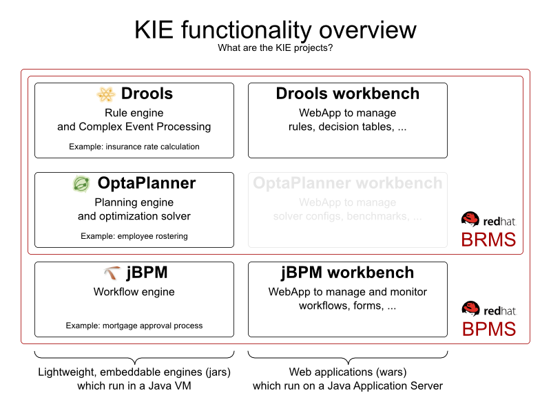
Red Hat sponsors OptaPlanner development by employing the core team. For enterprise support and consulting, take a look at the BRMS and BPMS products (which contain OptaPlanner) or contact Red Hat.
OptaPlanner is part of the KIE group of projects. It releases regularly (often once or twice per month) together with the Drools rule engine and the jBPM workflow engine.
See the architecture overview to learn more about the optional integration with Drools.
Suppose your company owns a number of cloud computers and needs to run a number of processes on those computers. Assign each process to a computer under the following four constraints.
The following hard constraints must be fulfilled:
Every computer must be able to handle the minimum hardware requirements of the sum of its processes:
The CPU power of a computer must be at least the sum of the CPU power required by the processes assigned to that computer.
The RAM memory of a computer must be at least the sum of the RAM memory required by the processes assigned to that computer.
The network bandwidth of a computer must be at least the sum of the network bandwidth required by the processes assigned to that computer.
The following soft constraints should be optimized:
Each computer that has one or more processes assigned, incurs a maintenance cost (which is fixed per computer).
Minimize the total maintenance cost.
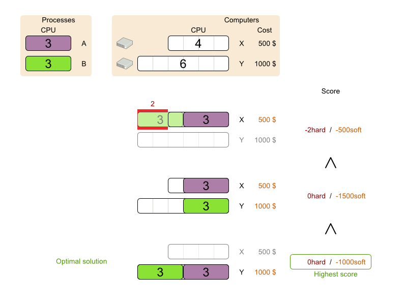
This problem is a form of bin packing. The following is a simplified example, where we assign four processes to two computers with two constraints (CPU and RAM) with a simple algorithm:
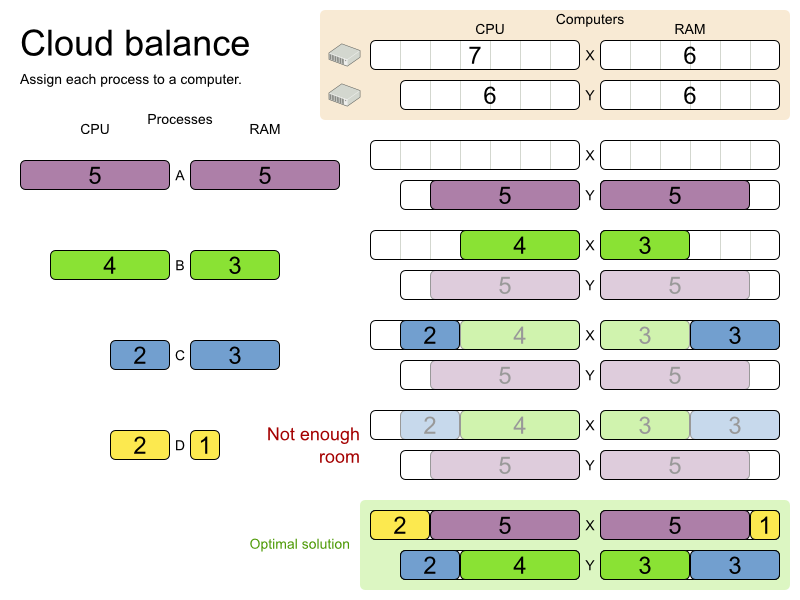
The simple algorithm used here is the First Fit Decreasing algorithm, which assigns the bigger processes first and assigns the smaller processes to the remaining space. As you can see, it is not optimal, as it does not leave enough room to assign the yellow process "D".
Planner does find the more optimal solution fast by using additional, smarter algorithms. It also scales: both in data (more processes, more computers) and constraints (more hardware requirements, other constraints). So see how Planner can be used in this scenario.
Table 2.1. Cloud Balancing Problem Size
| Problem Size | Computers | Processes | Search Space |
|---|---|---|---|
| 2computers-6processes | 2 | 6 | 64 |
| 3computers-9processes | 3 | 9 | 10^4 |
| 4computers-012processes | 4 | 12 | 10^7 |
| 100computers-300processes | 100 | 300 | 10^600 |
| 200computers-600processes | 200 | 600 | 10^1380 |
| 400computers-1200processes | 400 | 1200 | 10^3122 |
| 800computers-2400processes | 800 | 2400 | 10^6967 |
Beginning with the domain model:
Computer: represents a computer with certain hardware (CPU power, RAM memory, network bandwidth) and maintenance cost.Process: represents a process with a demand. Needs to be assigned to aComputerby Planner.CloudBalance: represents a problem. Contains everyComputerandProcessfor a certain data set.
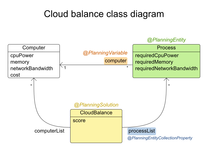
In the UML class diagram above, the Planner concepts are already annotated:
Planning entity: the class (or classes) that changes during planning. In this example, it is the class
Process.Planning variable: the property (or properties) of a planning entity class that changes during planning. In this example, it is the property
computeron the classProcess.Solution: the class that represents a data set and contains all planning entities. In this example that is the class
CloudBalance.
Try it yourself. Download and configure the examples in your
preferred IDE. Run org.optaplanner.examples.cloudbalancing.app.CloudBalancingHelloWorld.
By default, it is configured to run for 120 seconds. It will execute this code:
Example 2.1. CloudBalancingHelloWorld.java
public class CloudBalancingHelloWorld {

    public static void main(String[] args) {
        // Build the Solver
        SolverFactory solverFactory = SolverFactory.createFromXmlResource(
                "org/optaplanner/examples/cloudbalancing/solver/cloudBalancingSolverConfig.xml");
        Solver solver = solverFactory.buildSolver();

        // Load a problem with 400 computers and 1200 processes
        CloudBalance unsolvedCloudBalance = new CloudBalancingGenerator().createCloudBalance(400, 1200);

        // Solve the problem
        solver.solve(unsolvedCloudBalance);
        CloudBalance solvedCloudBalance = (CloudBalance) solver.getBestSolution();

        // Display the result
        System.out.println("\nSolved cloudBalance with 400 computers and 1200 processes:\n"
                + toDisplayString(solvedCloudBalance));
    }

    ...

}
The code example does the following:
Build the
Solverbased on a solver configuration (in this case an XML file from the classpath).SolverFactory solverFactory = SolverFactory.createFromXmlResource( "org/optaplanner/examples/cloudbalancing/solver/cloudBalancingSolverConfig.xml"); Solver solver = solverFactory.buildSolver();Load the problem.
CloudBalancingGeneratorgenerates a random problem: you will replace this with a class that loads a real problem, for example from a database.CloudBalance unsolvedCloudBalance = new CloudBalancingGenerator().createCloudBalance(400, 1200);Solve the problem.
        solver.solve(unsolvedCloudBalance);
        CloudBalance solvedCloudBalance = (CloudBalance) solver.getBestSolution();
Display the result.
        System.out.println("\nSolved cloudBalance with 400 computers and 1200 processes:\n"
                + toDisplayString(solvedCloudBalance));
The only complicated part is building the Solver, as detailed in the next section.
Take a look at the solver configuration:
Example 2.2. cloudBalancingSolverConfig.xml
<?xml version="1.0" encoding="UTF-8"?>
<solver>
  <!-- Domain model configuration -->
  <solutionClass>org.optaplanner.examples.cloudbalancing.domain.CloudBalance</solutionClass>
  <entityClass>org.optaplanner.examples.cloudbalancing.domain.CloudProcess</entityClass>

  <!-- Score configuration -->
  <scoreDirectorFactory>
    <scoreDefinitionType>HARD_SOFT</scoreDefinitionType>
    <easyScoreCalculatorClass>org.optaplanner.examples.cloudbalancing.solver.score.CloudBalancingEasyScoreCalculator</easyScoreCalculatorClass>
    <!--<scoreDrl>org/optaplanner/examples/cloudbalancing/solver/cloudBalancingScoreRules.drl</scoreDrl>-->
    <initializingScoreTrend>ONLY_DOWN</initializingScoreTrend>
  </scoreDirectorFactory>

  <!-- Optimization algorithms configuration -->
  <termination>
    <secondsSpentLimit>60</secondsSpentLimit>
  </termination>
</solver>
This solver configuration consists of three parts:
Domain model configuration: What can Planner change? We need to make Planner aware of our domain classes:
  <solutionClass>org.optaplanner.examples.cloudbalancing.domain.CloudBalance</solutionClass>
  <entityClass>org.optaplanner.examples.cloudbalancing.domain.CloudProcess</entityClass>
Score configuration: How should Planner optimize the planning variables? What is our goal? Since we have hard and soft constraints, we use a
HardSoftScore. But we also need to tell Planner how to calculate the score, depending on our business requirements. Further down, we will look into two alternatives to calculate the score: using a simple Java implementation, or using Drools DRL.<scoreDirectorFactory> <scoreDefinitionType>HARD_SOFT</scoreDefinitionType> <easyScoreCalculatorClass>org.optaplanner.examples.cloudbalancing.solver.score.CloudBalancingEasyScoreCalculator</easyScoreCalculatorClass> <!--<scoreDrl>org/optaplanner/examples/cloudbalancing/solver/cloudBalancingScoreRules.drl</scoreDrl>--> <initializingScoreTrend>ONLY_DOWN</initializingScoreTrend> </scoreDirectorFactory>Optimization algorithms configuration: How should Planner optimize it and for how long? In this case, we terminate it after 60 seconds and use the default optimization algorithms (because no explicit optimization algorithms are configured). The default algorithms should already easily surpass human planners and most in-house implementations. Use the Benchmarker to power tweak it to get even better results.
  <termination>
    <secondsSpentLimit>60</secondsSpentLimit>
  </termination>
Let's examine the domain model classes and the score configuration.
The Computer class is a POJO (Plain Old Java Object). Usually, you will have more of
this kind of classes.
Example 2.3. CloudComputer.java
public class CloudComputer ... {

    private int cpuPower;
    private int memory;
    private int networkBandwidth;
    private int cost;

    ... // getters
}The Process class is particularly important. We need to tell Planner that it can change
the field computer, so we annotate the class with @PlanningEntity and the
getter getComputer() with @PlanningVariable:
Example 2.4. CloudProcess.java
@PlanningEntity(...)
public class CloudProcess ... {

    private int requiredCpuPower;
    private int requiredMemory;
    private int requiredNetworkBandwidth;

    private CloudComputer computer;

    ... // getters

    @PlanningVariable(valueRangeProviderRefs = {"computerRange"})
    public CloudComputer getComputer() {
        return computer;
    }

    public void setComputer(CloudComputer computer) {
        computer = computer;
    }

    // ************************************************************************
    // Complex methods
    // ************************************************************************

    ...

}
The values that Planner can choose from for the field computer, are retrieved from a
method on the Solution implementation: CloudBalance.getComputerList(),
which returns a list of all computers in the current data set. The valueRangeProviderRefs
property is used to pass this information to the Planner.
Note
Instead of getter annotations, it is also possible to use field annotations.
The CloudBalance class implements the Solution interface. It holds
a list of all computers and processes. We need to tell Planner how to retrieve the collection of processes that
it can change, therefore we must annotate the getter getProcessList with
@PlanningEntityCollectionProperty.
The CloudBalance class also has a property score, which is the
Score of that Solution instance in its current state:
Example 2.5. CloudBalance.java
public class CloudBalance ... implements Solution<HardSoftScore> {

    private List<CloudComputer> computerList;

    private List<CloudProcess> processList;

    private HardSoftScore score;

    @ValueRangeProvider(id = "computerRange")
    public List<CloudComputer> getComputerList() {
        return computerList;
    }

    @PlanningEntityCollectionProperty
    public List<CloudProcess> getProcessList() {
        return processList;
    }

    ...

    public HardSoftScore getScore() {
        return score;
    }

    public void setScore(HardSoftScore score) {
        this.score = score;
    }

    // ************************************************************************
    // Complex methods
    // ************************************************************************

    public Collection<? extends Object> getProblemFacts() {
        List<Object> facts = new ArrayList<Object>();
        facts.addAll(computerList);
        // Do not add the planning entity's (processList) because that will be done automatically
        return facts;
    }

    ...

}
The getProblemFacts() method is only needed for score calculation with Drools. It is
not needed for the other score calculation types.
Planner will search for the Solution with the highest Score. This
example uses a HardSoftScore, which means Planner will look for the solution with no hard
constraints broken (fulfill hardware requirements) and as little as possible soft constraints broken (minimize
maintenance cost).
Of course, Planner needs to be told about these domain-specific score constraints. There are several ways to implement such a score function:
Easy Java
Incremental Java
Drools
Let's take a look at two different implementations:
One way to define a score function is to implement the interface EasyScoreCalculator in
plain Java.
  <scoreDirectorFactory>
    <scoreDefinitionType>HARD_SOFT</scoreDefinitionType>
    <easyScoreCalculatorClass>org.optaplanner.examples.cloudbalancing.solver.score.CloudBalancingEasyScoreCalculator</easyScoreCalculatorClass>
  </scoreDirectorFactory>
Just implement the calculateScore(Solution) method to return a
HardSoftScore instance.
Example 2.6. CloudBalancingEasyScoreCalculator.java
public class CloudBalancingEasyScoreCalculator implements EasyScoreCalculator<CloudBalance> {

    /**
     * A very simple implementation. The double loop can easily be removed by using Maps as shown in
     * {@link CloudBalancingMapBasedEasyScoreCalculator#calculateScore(CloudBalance)}.
     */
    public HardSoftScore calculateScore(CloudBalance cloudBalance) {
        int hardScore = 0;
        int softScore = 0;
        for (CloudComputer computer : cloudBalance.getComputerList()) {
            int cpuPowerUsage = 0;
            int memoryUsage = 0;
            int networkBandwidthUsage = 0;
            boolean used = false;

            // Calculate usage
            for (CloudProcess process : cloudBalance.getProcessList()) {
                if (computer.equals(process.getComputer())) {
                    cpuPowerUsage += process.getRequiredCpuPower();
                    memoryUsage += process.getRequiredMemory();
                    networkBandwidthUsage += process.getRequiredNetworkBandwidth();
                    used = true;
                }
            }

            // Hard constraints
            int cpuPowerAvailable = computer.getCpuPower() - cpuPowerUsage;
            if (cpuPowerAvailable < 0) {
                hardScore += cpuPowerAvailable;
            }
            int memoryAvailable = computer.getMemory() - memoryUsage;
            if (memoryAvailable < 0) {
                hardScore += memoryAvailable;
            }
            int networkBandwidthAvailable = computer.getNetworkBandwidth() - networkBandwidthUsage;
            if (networkBandwidthAvailable < 0) {
                hardScore += networkBandwidthAvailable;
            }

            // Soft constraints
            if (used) {
                softScore -= computer.getCost();
            }
        }
        return HardSoftScore.valueOf(hardScore, softScore);
    }

}
Even if we optimize the code above to use Maps to iterate through the
processList only once, it is still slow because it does not
do incremental score calculation. To fix that, either use an incremental Java score function or a Drools score
function. Let's take a look at the latter.
To use the Drools rule engine as a score function, simply add a scoreDrl resource in
the classpath:
  <scoreDirectorFactory>
    <scoreDefinitionType>HARD_SOFT</scoreDefinitionType>
    <scoreDrl>org/optaplanner/examples/cloudbalancing/solver/cloudBalancingScoreRules.drl</scoreDrl>
  </scoreDirectorFactory>
First, we want to make sure that all computers have enough CPU, RAM and network bandwidth to support all their processes, so we make these hard constraints:
Example 2.7. cloudBalancingScoreRules.drl - Hard Constraints
...

import org.optaplanner.examples.cloudbalancing.domain.CloudBalance;
import org.optaplanner.examples.cloudbalancing.domain.CloudComputer;
import org.optaplanner.examples.cloudbalancing.domain.CloudProcess;

global HardSoftScoreHolder scoreHolder;

// ############################################################################
// Hard constraints
// ############################################################################

rule "requiredCpuPowerTotal"
    when
        $computer : CloudComputer($cpuPower : cpuPower)
        $requiredCpuPowerTotal : Number(intValue > $cpuPower) from accumulate(
            CloudProcess(
                computer == $computer,
                $requiredCpuPower : requiredCpuPower),
            sum($requiredCpuPower)
        )
    then
        scoreHolder.addHardConstraintMatch(kcontext, $cpuPower - $requiredCpuPowerTotal.intValue());
end

rule "requiredMemoryTotal"
    ...
end

rule "requiredNetworkBandwidthTotal"
    ...
end
Next, if those constraints are met, we want to minimize the maintenance cost, so we add that as a soft constraint:
Example 2.8. cloudBalancingScoreRules.drl - Soft Constraints
// ############################################################################
// Soft constraints
// ############################################################################

rule "computerCost"
    when
        $computer : CloudComputer($cost : cost)
        exists CloudProcess(computer == $computer)
    then
        scoreHolder.addSoftConstraintMatch(kcontext, - $cost);
end
If you use the Drools rule engine for score calculation, you can integrate with other Drools technologies, such as decision tables (XLS or web based), the KIE Workbench, ...
Now that this simple example works, try going further. Enrich the domain model and add extra constraints such as these:
Each
Processbelongs to aService. A computer might crash, so processes running the same service should be assigned to different computers.Each
Computeris located in aBuilding. A building might burn down, so processes of the same services should be assigned to computers in different buildings.
Planner has several examples. In this manual we explain mainly using the n queens example and cloud balancing example. So it's advisable to read at least those sections.
The source code of all these examples is available in the distribution zip under
examples/sources and also in git under
optaplanner/optaplanner-examples.
Table 3.1. Examples Overview
| Example | Domain | Size | Competition? | Special features used |
|---|---|---|---|---|
| N queens |
|
|
| None |
| Cloud balancing |
|
|
| |
| Traveling salesman |
|
|
| |
| Dinner party |
|
|
|
|
| Tennis club scheduling |
|
|
| |
| Course timetabling |
|
|
| |
| Machine reassignment |
|
|
| |
| Vehicle routing |
|
|
|
|
| Vehicle routing with time windows | Extra on Vehicle routing:
|
|
| Extra on Vehicle routing:
|
| Project job scheduling |
|
|
| |
| Hospital bed planning |
|
|
| |
| Exam timetabling |
|
|
|
|
| Employee rostering |
|
|
| |
| Traveling tournament |
|
|
|
|
| Cheap time scheduling |
|
|
|
A realistic competition is an official, independent competition:
that clearly defines a real-word use case
with real-world constraints
with multiple, real-world datasets
that expects reproducible results within a specific time limit on specific hardware
that has had serious participation from the academic and/or enterprise Operations Research community
These realistic competitions provide an objective comparison of Planner with competitive software and academic research.
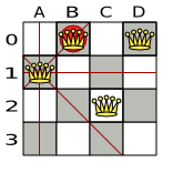
Place n queens on a n sized chessboard so no 2 queens can attack each other. The most common n queens puzzle is the 8 queens puzzle, with n = 8:
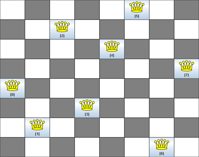
Constraints:
Use a chessboard of n columns and n rows.
Place n queens on the chessboard.
No 2 queens can attack each other. A queen can attack any other queen on the same horizontal, vertical or diagonal line.
This documentation heavily uses the 4 queens puzzle as the primary example.
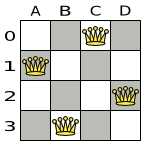
A proposed solution could be:
The above solution is wrong because queens A1 and B0 can attack each
other (so can queens B0 and D0). Removing queen B0
would respect the "no 2 queens can attack each other" constraint, but would break the "place n queens"
constraint.
Below is a correct solution:
All the constraints have been met, so the solution is correct. Note that most n queens puzzles have multiple correct solutions. We'll focus on finding a single correct solution for a given n, not on finding the number of possible correct solutions for a given n.
4queens   has   4 queens with a search space of    256.
8queens   has   8 queens with a search space of   10^7.
16queens  has  16 queens with a search space of  10^19.
32queens  has  32 queens with a search space of  10^48.
64queens  has  64 queens with a search space of 10^115.
256queens has 256 queens with a search space of 10^616.
The implementation of the N queens example has not been optimized because it functions as a beginner example. Nevertheless, it can easily handle 64 queens. With a few changes it has been shown to easily handle 5000 queens and more.
Use a good domain model: it will be easier to understand and solve your planning problem. This is the domain model for the n queens example:
public class Column {

    private int index;

    // ... getters and setters
}
public class Row {
private int index;
// ... getters and setters
}public class Queen {
private Column column;
private Row row;
public int getAscendingDiagonalIndex() {...}
public int getDescendingDiagonalIndex() {...}
// ... getters and setters
}A Queen instance has a Column (for example: 0 is column A, 1 is
column B, ...) and a Row (its row, for example: 0 is row 0, 1 is row 1, ...). Based on the
column and the row, the ascending diagonal line as well as the descending diagonal line can be calculated. The
column and row indexes start from the upper left corner of the chessboard.
public class NQueens implements Solution<SimpleScore> {

    private int n;
    private List<Column> columnList;
    private List<Row> rowList;

    private List<Queen> queenList;

    private SimpleScore score;

    // ... getters and setters
}
A single NQueens instance contains a list of all Queen instances. It
is the Solution implementation which will be supplied to, solved by and retrieved from the
Solver. Notice that in the 4 queens example, NQueens's getN() method will always return
4.
Table 3.2. A Solution for 4 Queens Shown in the Domain Model
| A solution | Queen | columnIndex | rowIndex | ascendingDiagonalIndex (columnIndex + rowIndex) | descendingDiagonalIndex (columnIndex - rowIndex) |
|---|---|---|---|---|---|
 | A1 | 0 | 1 | 1 (**) | -1 |
| B0 | 1 | 0 (*) | 1 (**) | 1 | |
| C2 | 2 | 2 | 4 | 0 | |
| D0 | 3 | 0 (*) | 3 | 3 |
When 2 queens share the same column, row or diagonal line, such as (*) and (**), they can attack each other.
This example is explained in a tutorial.
Given a list of cities, find the shortest tour for a salesman that visits each city exactly once.
The problem is defined by Wikipedia. It is one of the most intensively studied problems in computational mathematics. Yet, in the real world, it's often only part of a planning problem, along with other constraints, such as employee shift rostering constraints.
dj38     has  38 cities with a search space of   10^58.
europe40 has  40 cities with a search space of   10^62.
st70     has  70 cities with a search space of  10^126.
pcb442   has 442 cities with a search space of 10^1166.
lu980    has 980 cities with a search space of 10^2927.
Miss Manners is throwing another dinner party.
This time she invited 144 guests and prepared 12 round tables with 12 seats each.
Every guest should sit next to someone (left and right) of the opposite gender.
And that neighbour should have at least one hobby in common with the guest.
At every table, there should be 2 politicians, 2 doctors, 2 socialites, 2 coaches, 2 teachers and 2 programmers.
And the 2 politicians, 2 doctors, 2 coaches and 2 programmers shouldn't be the same kind at a table.
Drools Expert also has the normal Miss Manners example (which is much smaller) and employs an exhaustive heuristic to solve it. Planner's implementation is far more scalable because it uses heuristics to find the best solution and Drools Expert to calculate the score of each solution.
Every week the tennis club has 4 teams playing round robin against each other. Assign those 4 spots to the teams fairly.
Hard constraints:
Conflict: A team can only play once per day.
Unavailability: Some teams are unavailable on some dates.
Medium constraints:
Fair assignment: All teams should play an (almost) equal number of times.
Soft constraints:
Evenly confrontation: Each team should play against every other team an equal number of times.
munich-7teams has 7 teams, 18 days, 12 unavailabilityPenalties and 72 teamAssignments with a search space of 10^60.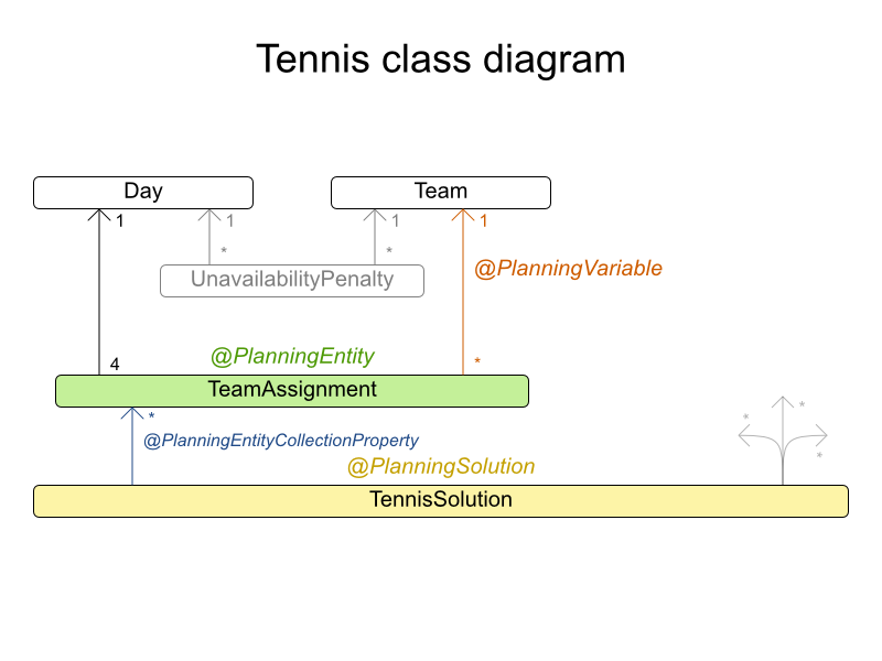
Schedule each lecture into a timeslot and into a room.
Hard constraints:
Teacher conflict: A teacher must not have 2 lectures in the same period.
Curriculum conflict: A curriculum must not have 2 lectures in the same period.
Room occupancy: 2 lectures must not be in the same room in the same period.
Unavailable period (specified per dataset): A specific lecture must not be assigned to a specific period.
Soft constraints:
Room capacity: A room's capacity should not be less than the number of students in its lecture.
Minimum working days: Lectures of the same course should be spread out into a minimum number of days.
Curriculum compactness: Lectures belonging to the same curriculum should be adjacent to each other (so in consecutive periods).
Room stability: Lectures of the same course should be assigned the same room.
The problem is defined by the International Timetabling Competition 2007 track 3.
comp01 has 24 teachers,  14 curricula,  30 courses, 160 lectures, 30 periods,  6 rooms and   53 unavailable period constraints with a search space of  10^360.
comp02 has 71 teachers,  70 curricula,  82 courses, 283 lectures, 25 periods, 16 rooms and  513 unavailable period constraints with a search space of  10^736.
comp03 has 61 teachers,  68 curricula,  72 courses, 251 lectures, 25 periods, 16 rooms and  382 unavailable period constraints with a search space of  10^653.
comp04 has 70 teachers,  57 curricula,  79 courses, 286 lectures, 25 periods, 18 rooms and  396 unavailable period constraints with a search space of  10^758.
comp05 has 47 teachers, 139 curricula,  54 courses, 152 lectures, 36 periods,  9 rooms and  771 unavailable period constraints with a search space of  10^381.
comp06 has 87 teachers,  70 curricula, 108 courses, 361 lectures, 25 periods, 18 rooms and  632 unavailable period constraints with a search space of  10^957.
comp07 has 99 teachers,  77 curricula, 131 courses, 434 lectures, 25 periods, 20 rooms and  667 unavailable period constraints with a search space of 10^1171.
comp08 has 76 teachers,  61 curricula,  86 courses, 324 lectures, 25 periods, 18 rooms and  478 unavailable period constraints with a search space of  10^859.
comp09 has 68 teachers,  75 curricula,  76 courses, 279 lectures, 25 periods, 18 rooms and  405 unavailable period constraints with a search space of  10^740.
comp10 has 88 teachers,  67 curricula, 115 courses, 370 lectures, 25 periods, 18 rooms and  694 unavailable period constraints with a search space of  10^981.
comp11 has 24 teachers,  13 curricula,  30 courses, 162 lectures, 45 periods,  5 rooms and   94 unavailable period constraints with a search space of  10^381.
comp12 has 74 teachers, 150 curricula,  88 courses, 218 lectures, 36 periods, 11 rooms and 1368 unavailable period constraints with a search space of  10^566.
comp13 has 77 teachers,  66 curricula,  82 courses, 308 lectures, 25 periods, 19 rooms and  468 unavailable period constraints with a search space of  10^824.
comp14 has 68 teachers,  60 curricula,  85 courses, 275 lectures, 25 periods, 17 rooms and  486 unavailable period constraints with a search space of  10^722.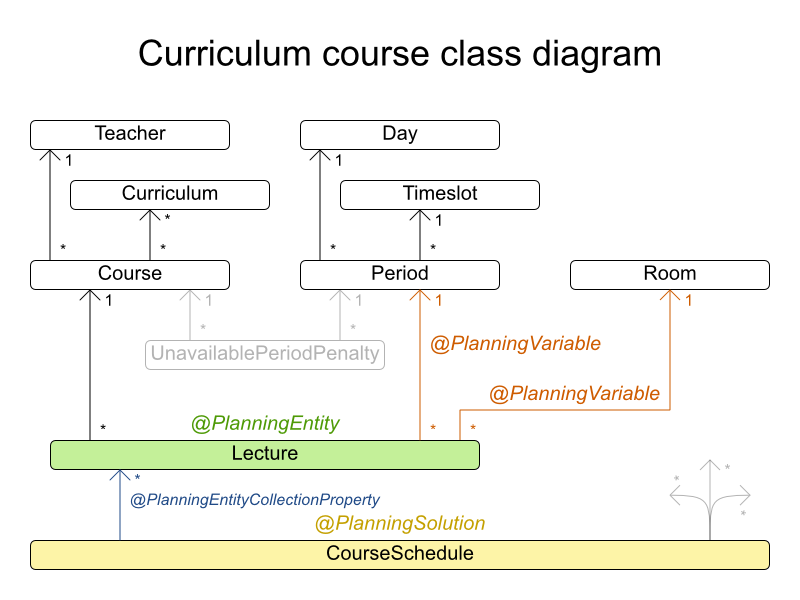
Assign each process to a machine. All processes already have an original (unoptimized) assignment. Each process requires an amount of each resource (such as CPU, RAM, ...). This is a more complex version of the Cloud Balancing example.
Hard constraints:
Maximum capacity: The maximum capacity for each resource for each machine must not be exceeded.
Conflict: Processes of the same service must run on distinct machines.
Spread: Processes of the same service must be spread out across locations.
Dependency: The processes of a service depending on another service must run in the neighborhood of a process of the other service.
Transient usage: Some resources are transient and count towards the maximum capacity of both the original machine as the newly assigned machine.
Soft constraints:
Load: The safety capacity for each resource for each machine should not be exceeded.
Balance: Leave room for future assignments by balancing the available resources on each machine.
Process move cost: A process has a move cost.
Service move cost: A service has a move cost.
Machine move cost: Moving a process from machine A to machine B has another A-B specific move cost.
The problem is defined by the Google ROADEF/EURO Challenge 2012.
model_a1_1 has  2 resources,  1 neighborhoods,   4 locations,    4 machines,    79 services,   100 processes and 1 balancePenalties with a search space of     10^60.
model_a1_2 has  4 resources,  2 neighborhoods,   4 locations,  100 machines,   980 services,  1000 processes and 0 balancePenalties with a search space of   10^2000.
model_a1_3 has  3 resources,  5 neighborhoods,  25 locations,  100 machines,   216 services,  1000 processes and 0 balancePenalties with a search space of   10^2000.
model_a1_4 has  3 resources, 50 neighborhoods,  50 locations,   50 machines,   142 services,  1000 processes and 1 balancePenalties with a search space of   10^1698.
model_a1_5 has  4 resources,  2 neighborhoods,   4 locations,   12 machines,   981 services,  1000 processes and 1 balancePenalties with a search space of   10^1079.
model_a2_1 has  3 resources,  1 neighborhoods,   1 locations,  100 machines,  1000 services,  1000 processes and 0 balancePenalties with a search space of   10^2000.
model_a2_2 has 12 resources,  5 neighborhoods,  25 locations,  100 machines,   170 services,  1000 processes and 0 balancePenalties with a search space of   10^2000.
model_a2_3 has 12 resources,  5 neighborhoods,  25 locations,  100 machines,   129 services,  1000 processes and 0 balancePenalties with a search space of   10^2000.
model_a2_4 has 12 resources,  5 neighborhoods,  25 locations,   50 machines,   180 services,  1000 processes and 1 balancePenalties with a search space of   10^1698.
model_a2_5 has 12 resources,  5 neighborhoods,  25 locations,   50 machines,   153 services,  1000 processes and 0 balancePenalties with a search space of   10^1698.
model_b_1  has 12 resources,  5 neighborhoods,  10 locations,  100 machines,  2512 services,  5000 processes and 0 balancePenalties with a search space of  10^10000.
model_b_2  has 12 resources,  5 neighborhoods,  10 locations,  100 machines,  2462 services,  5000 processes and 1 balancePenalties with a search space of  10^10000.
model_b_3  has  6 resources,  5 neighborhoods,  10 locations,  100 machines, 15025 services, 20000 processes and 0 balancePenalties with a search space of  10^40000.
model_b_4  has  6 resources,  5 neighborhoods,  50 locations,  500 machines,  1732 services, 20000 processes and 1 balancePenalties with a search space of  10^53979.
model_b_5  has  6 resources,  5 neighborhoods,  10 locations,  100 machines, 35082 services, 40000 processes and 0 balancePenalties with a search space of  10^80000.
model_b_6  has  6 resources,  5 neighborhoods,  50 locations,  200 machines, 14680 services, 40000 processes and 1 balancePenalties with a search space of  10^92041.
model_b_7  has  6 resources,  5 neighborhoods,  50 locations, 4000 machines, 15050 services, 40000 processes and 1 balancePenalties with a search space of 10^144082.
model_b_8  has  3 resources,  5 neighborhoods,  10 locations,  100 machines, 45030 services, 50000 processes and 0 balancePenalties with a search space of 10^100000.
model_b_9  has  3 resources,  5 neighborhoods, 100 locations, 1000 machines,  4609 services, 50000 processes and 1 balancePenalties with a search space of 10^150000.
model_b_10 has  3 resources,  5 neighborhoods, 100 locations, 5000 machines,  4896 services, 50000 processes and 1 balancePenalties with a search space of 10^184948.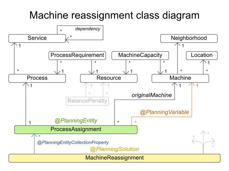
Using a fleet of vehicles, pick up the objects of each customer and bring them to the depot. Each vehicle can service multiple customers, but it has a limited capacity.
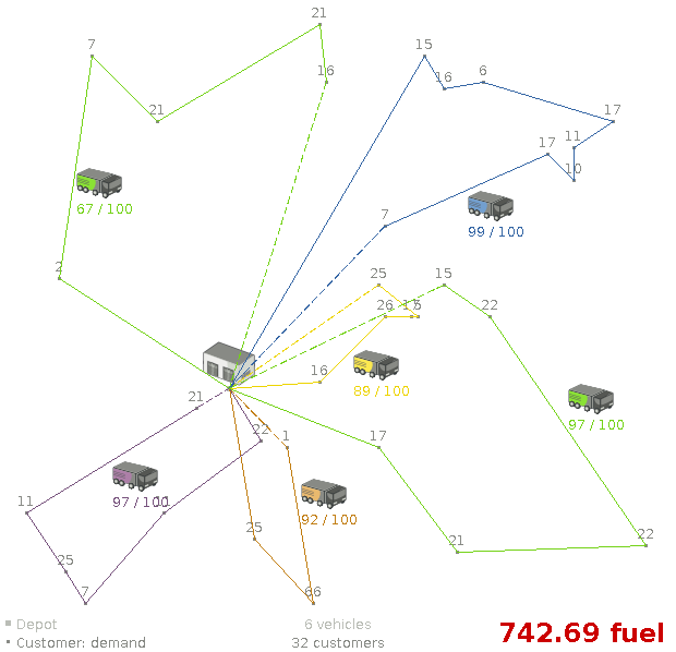
Besides the basic case (CVRP), there is also a variant with time windows (CVRPTW).
Hard constraints:
Vehicle capacity: a vehicle cannot carry more items then its capacity.
Time windows (only in CVRPTW):
Travel time: Traveling from one location to another takes time.
Customer service duration: a vehicle must stay at the customer for the length of the service duration.
Customer ready time: a vehicle may arrive before the customer's ready time, but it must wait until the ready time before servicing.
Customer due time: a vehicle must arrive on time, before the customer's due time.
Soft constraints:
Total distance: minimize the total distance driven (fuel consumption) of all vehicles.
The capacitated vehicle routing problem (CVRP) and its timewindowed variant (CVRPTW) are defined by the VRP web.
CVRP instances (without time windows):
A-n32-k5  has 1 depots,  5 vehicles and  31 customers with a search space of  10^46.
A-n33-k5  has 1 depots,  5 vehicles and  32 customers with a search space of  10^48.
A-n33-k6  has 1 depots,  6 vehicles and  32 customers with a search space of  10^48.
A-n34-k5  has 1 depots,  5 vehicles and  33 customers with a search space of  10^50.
A-n36-k5  has 1 depots,  5 vehicles and  35 customers with a search space of  10^54.
A-n37-k5  has 1 depots,  5 vehicles and  36 customers with a search space of  10^56.
A-n37-k6  has 1 depots,  6 vehicles and  36 customers with a search space of  10^56.
A-n38-k5  has 1 depots,  5 vehicles and  37 customers with a search space of  10^58.
A-n39-k5  has 1 depots,  5 vehicles and  38 customers with a search space of  10^60.
A-n39-k6  has 1 depots,  6 vehicles and  38 customers with a search space of  10^60.
A-n44-k7  has 1 depots,  7 vehicles and  43 customers with a search space of  10^70.
A-n45-k6  has 1 depots,  6 vehicles and  44 customers with a search space of  10^72.
A-n45-k7  has 1 depots,  7 vehicles and  44 customers with a search space of  10^72.
A-n46-k7  has 1 depots,  7 vehicles and  45 customers with a search space of  10^74.
A-n48-k7  has 1 depots,  7 vehicles and  47 customers with a search space of  10^78.
A-n53-k7  has 1 depots,  7 vehicles and  52 customers with a search space of  10^89.
A-n54-k7  has 1 depots,  7 vehicles and  53 customers with a search space of  10^91.
A-n55-k9  has 1 depots,  9 vehicles and  54 customers with a search space of  10^93.
A-n60-k9  has 1 depots,  9 vehicles and  59 customers with a search space of 10^104.
A-n61-k9  has 1 depots,  9 vehicles and  60 customers with a search space of 10^106.
A-n62-k8  has 1 depots,  8 vehicles and  61 customers with a search space of 10^108.
A-n63-k10 has 1 depots, 10 vehicles and  62 customers with a search space of 10^111.
A-n63-k9  has 1 depots,  9 vehicles and  62 customers with a search space of 10^111.
A-n64-k9  has 1 depots,  9 vehicles and  63 customers with a search space of 10^113.
A-n65-k9  has 1 depots,  9 vehicles and  64 customers with a search space of 10^115.
A-n69-k9  has 1 depots,  9 vehicles and  68 customers with a search space of 10^124.
A-n80-k10 has 1 depots, 10 vehicles and  79 customers with a search space of 10^149.
F-n135-k7 has 1 depots,  7 vehicles and 134 customers with a search space of 10^285.
F-n45-k4  has 1 depots,  4 vehicles and  44 customers with a search space of  10^72.
F-n72-k4  has 1 depots,  4 vehicles and  71 customers with a search space of 10^131.
CVRPTW instances (with time windows):
Solomon_025_C101       has 1 depots,  25 vehicles and   25 customers with a search space of   10^34.
Solomon_025_C201       has 1 depots,  25 vehicles and   25 customers with a search space of   10^34.
Solomon_025_R101       has 1 depots,  25 vehicles and   25 customers with a search space of   10^34.
Solomon_025_R201       has 1 depots,  25 vehicles and   25 customers with a search space of   10^34.
Solomon_025_RC101      has 1 depots,  25 vehicles and   25 customers with a search space of   10^34.
Solomon_025_RC201      has 1 depots,  25 vehicles and   25 customers with a search space of   10^34.
Solomon_100_C101       has 1 depots,  25 vehicles and  100 customers with a search space of  10^200.
Solomon_100_C201       has 1 depots,  25 vehicles and  100 customers with a search space of  10^200.
Solomon_100_R101       has 1 depots,  25 vehicles and  100 customers with a search space of  10^200.
Solomon_100_R201       has 1 depots,  25 vehicles and  100 customers with a search space of  10^200.
Solomon_100_RC101      has 1 depots,  25 vehicles and  100 customers with a search space of  10^200.
Solomon_100_RC201      has 1 depots,  25 vehicles and  100 customers with a search space of  10^200.
Homberger_0200_C1_2_1  has 1 depots,  50 vehicles and  200 customers with a search space of  10^460.
Homberger_0200_C2_2_1  has 1 depots,  50 vehicles and  200 customers with a search space of  10^460.
Homberger_0200_R1_2_1  has 1 depots,  50 vehicles and  200 customers with a search space of  10^460.
Homberger_0200_R2_2_1  has 1 depots,  50 vehicles and  200 customers with a search space of  10^460.
Homberger_0200_RC1_2_1 has 1 depots,  50 vehicles and  200 customers with a search space of  10^460.
Homberger_0200_RC2_2_1 has 1 depots,  50 vehicles and  200 customers with a search space of  10^460.
Homberger_0400_C1_4_1  has 1 depots, 100 vehicles and  400 customers with a search space of 10^1040.
Homberger_0400_C2_4_1  has 1 depots, 100 vehicles and  400 customers with a search space of 10^1040.
Homberger_0400_R1_4_1  has 1 depots, 100 vehicles and  400 customers with a search space of 10^1040.
Homberger_0400_R2_4_1  has 1 depots, 100 vehicles and  400 customers with a search space of 10^1040.
Homberger_0400_RC1_4_1 has 1 depots, 100 vehicles and  400 customers with a search space of 10^1040.
Homberger_0400_RC2_4_1 has 1 depots, 100 vehicles and  400 customers with a search space of 10^1040.
Homberger_0600_C1_6_1  has 1 depots, 150 vehicles and  600 customers with a search space of 10^1666.
Homberger_0600_C2_6_1  has 1 depots, 150 vehicles and  600 customers with a search space of 10^1666.
Homberger_0600_R1_6_1  has 1 depots, 150 vehicles and  600 customers with a search space of 10^1666.
Homberger_0600_R2_6_1  has 1 depots, 150 vehicles and  600 customers with a search space of 10^1666.
Homberger_0600_RC1_6_1 has 1 depots, 150 vehicles and  600 customers with a search space of 10^1666.
Homberger_0600_RC2_6_1 has 1 depots, 150 vehicles and  600 customers with a search space of 10^1666.
Homberger_0800_C1_8_1  has 1 depots, 200 vehicles and  800 customers with a search space of 10^2322.
Homberger_0800_C2_8_1  has 1 depots, 200 vehicles and  800 customers with a search space of 10^2322.
Homberger_0800_R1_8_1  has 1 depots, 200 vehicles and  800 customers with a search space of 10^2322.
Homberger_0800_R2_8_1  has 1 depots, 200 vehicles and  800 customers with a search space of 10^2322.
Homberger_0800_RC1_8_1 has 1 depots, 200 vehicles and  800 customers with a search space of 10^2322.
Homberger_0800_RC2_8_1 has 1 depots, 200 vehicles and  800 customers with a search space of 10^2322.
Homberger_1000_C110_1  has 1 depots, 250 vehicles and 1000 customers with a search space of 10^3000.
Homberger_1000_C210_1  has 1 depots, 250 vehicles and 1000 customers with a search space of 10^3000.
Homberger_1000_R110_1  has 1 depots, 250 vehicles and 1000 customers with a search space of 10^3000.
Homberger_1000_R210_1  has 1 depots, 250 vehicles and 1000 customers with a search space of 10^3000.
Homberger_1000_RC110_1 has 1 depots, 250 vehicles and 1000 customers with a search space of 10^3000.
Homberger_1000_RC210_1 has 1 depots, 250 vehicles and 1000 customers with a search space of 10^3000.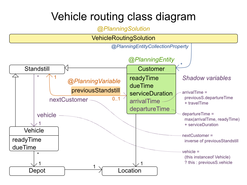
The vehicle routing with timewindows domain model makes heavily use of shadow variables. This allows it to express its constraints more naturally,
because properties such as arrivalTime and departureTime, are directly
available on the domain model.
In the real world, vehicles can't follow a straight line from location to location: they have to use roads and highways. From a business point of view, this matters a lot:
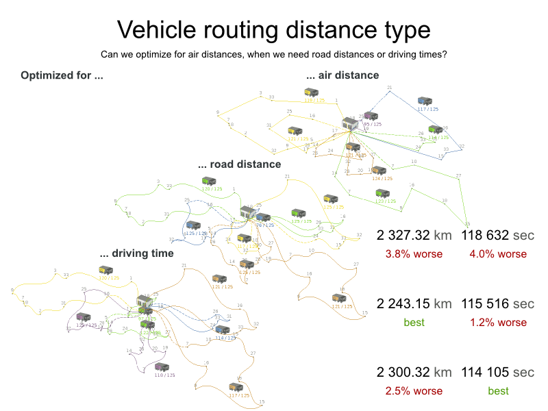
For the optimization algorithm, this doesn't matter much, as long as the distance between 2 points can be looked up (and are preferably precalculated). The road cost doesn't even need to be a distance, it can also be travel time, fuel cost, or a weighted function of those. There are several technologies available to precalculate road costs, such as GraphHopper (embeddable, offline Java engine), Open MapQuest (web service) and Google Maps Client API (web service).
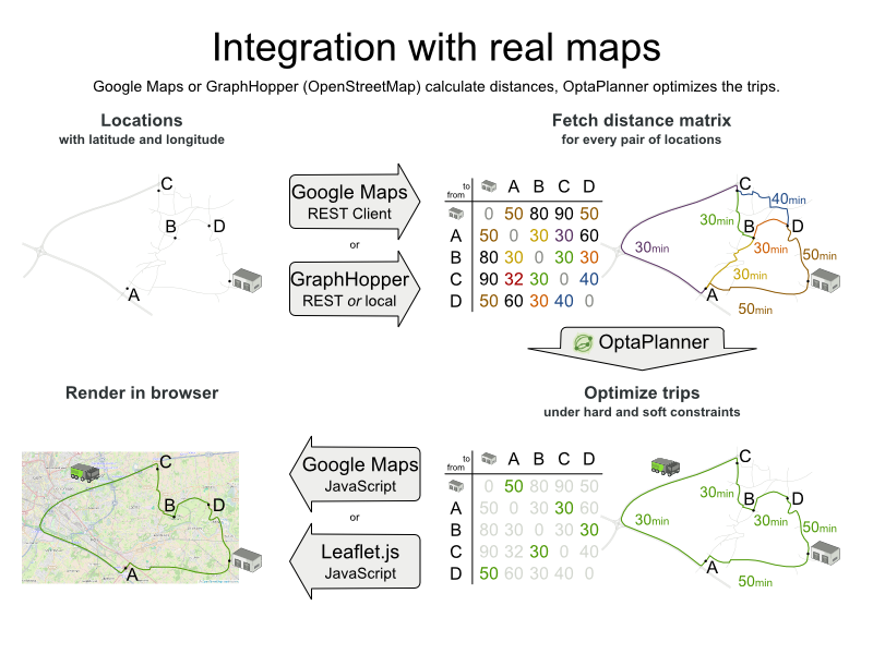
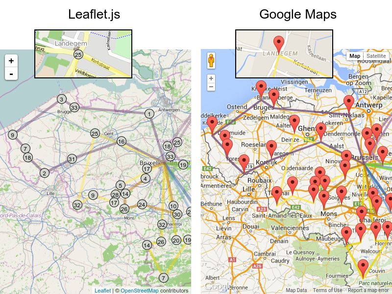
There are also several technologies to render it, such as Leaflet and Google Maps for developers: the
optaplanner-webexamples-*.war has an example which demonstrates such rendering:
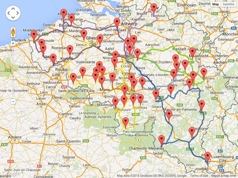
It's even possible to render the actual road routes with GraphHopper or Google Map Directions, but because of route overlaps on highways, it can become harder to see the standstill order:
Take special care that the road costs between 2 points use the same optimization criteria as the one used in Planner. For example, GraphHopper etc will by default return the fastest route, not the shortest route. Don't use the km (or miles) distances of the fastest GPS routes to optimize the shortest trip in Planner: this leads to a suboptimal solution as shown below:
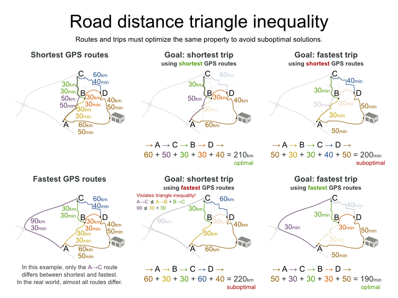
Contrary to popular belief, most users don't want the shortest route: they want the fastest route instead. They prefer highways over normal roads. They prefer normal roads over dirt roads. In the real world, the fastest and shortest route are rarely the same.
Schedule all jobs in time and execution mode to minimize project delays. Each job is part of a project. A job can be executed in different ways: each way is an execution mode that implies a different duration but also different resource usages. This is a form of flexible job shop scheduling.
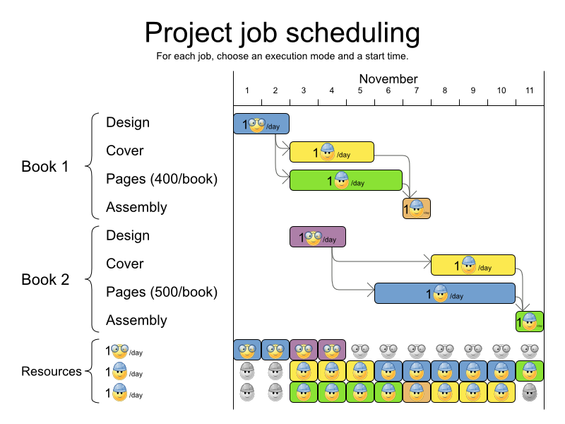
Hard constraints:
Job precedence: a job can only start when all its predecessor jobs are finished.
Resource capacity: do not use more resources then available.
Resources are local (shared between jobs of the same project) or global (shared between all jobs)
Resource are renewable (capacity available per day) or nonrenewable (capacity available for all days)
Medium constraints:
Total project delay: minimize the duration (makespan) of each project.
Soft constraints:
Total makespan: minimize the duration of the whole multi-project schedule.
The problem is defined by the MISTA 2013 challenge.
Schedule A-1  has  2 projects,  24 jobs,   64 execution modes,  7 resources and  150 resource requirements.
Schedule A-2  has  2 projects,  44 jobs,  124 execution modes,  7 resources and  420 resource requirements.
Schedule A-3  has  2 projects,  64 jobs,  184 execution modes,  7 resources and  630 resource requirements.
Schedule A-4  has  5 projects,  60 jobs,  160 execution modes, 16 resources and  390 resource requirements.
Schedule A-5  has  5 projects, 110 jobs,  310 execution modes, 16 resources and  900 resource requirements.
Schedule A-6  has  5 projects, 160 jobs,  460 execution modes, 16 resources and 1440 resource requirements.
Schedule A-7  has 10 projects, 120 jobs,  320 execution modes, 22 resources and  900 resource requirements.
Schedule A-8  has 10 projects, 220 jobs,  620 execution modes, 22 resources and 1860 resource requirements.
Schedule A-9  has 10 projects, 320 jobs,  920 execution modes, 31 resources and 2880 resource requirements.
Schedule A-10 has 10 projects, 320 jobs,  920 execution modes, 31 resources and 2970 resource requirements.
Schedule B-1  has 10 projects, 120 jobs,  320 execution modes, 31 resources and  900 resource requirements.
Schedule B-2  has 10 projects, 220 jobs,  620 execution modes, 22 resources and 1740 resource requirements.
Schedule B-3  has 10 projects, 320 jobs,  920 execution modes, 31 resources and 3060 resource requirements.
Schedule B-4  has 15 projects, 180 jobs,  480 execution modes, 46 resources and 1530 resource requirements.
Schedule B-5  has 15 projects, 330 jobs,  930 execution modes, 46 resources and 2760 resource requirements.
Schedule B-6  has 15 projects, 480 jobs, 1380 execution modes, 46 resources and 4500 resource requirements.
Schedule B-7  has 20 projects, 240 jobs,  640 execution modes, 61 resources and 1710 resource requirements.
Schedule B-8  has 20 projects, 440 jobs, 1240 execution modes, 42 resources and 3180 resource requirements.
Schedule B-9  has 20 projects, 640 jobs, 1840 execution modes, 61 resources and 5940 resource requirements.
Schedule B-10 has 20 projects, 460 jobs, 1300 execution modes, 42 resources and 4260 resource requirements.Assign each patient (that will come to the hospital) into a bed for each night that the patient will stay in the hospital. Each bed belongs to a room and each room belongs to a department. The arrival and departure dates of the patients is fixed: only a bed needs to be assigned for each night.
This problem features overconstrained datasets.
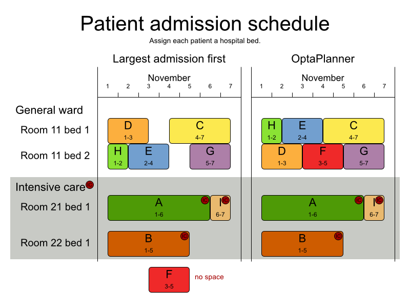
Hard constraints:
2 patients must not be assigned to the same bed in the same night. Weight:
-1000hard * conflictNightCount.A room can have a gender limitation: only females, only males, the same gender in the same night or no gender limitation at all. Weight:
-50hard * nightCount.A department can have a minimum or maximum age. Weight:
-100hard * nightCount.A patient can require a room with specific equipment(s). Weight:
-50hard *
            nightCount
.
Medium constraints:
Assign every patient to a bed, unless the dataset is overconstrained. Weight:
-1medium *
            nightCount
.
Soft constraints:
A patient can prefer a maximum room size, for example if he/she wants a single room. Weight:
-8soft * nightCount.A patient is best assigned to a department that specializes in his/her problem. Weight:
-10soft * nightCount.A patient is best assigned to a room that specializes in his/her problem. Weight:
-20soft * nightCount.That room speciality should be priority 1. Weight:
-10soft * (priority - 1) *
                nightCount
.
A patient can prefer a room with specific equipment(s). Weight:
-20soft *
            nightCount
.
The problem is a variant on Kaho's Patient Scheduling and the datasets come from real world hospitals.
testdata01 has 4 specialisms, 2 equipments, 4 departments,  98 rooms, 286 beds, 14 nights,  652 patients and  652 admissions with a search space of 10^1601.
testdata02 has 6 specialisms, 2 equipments, 6 departments, 151 rooms, 465 beds, 14 nights,  755 patients and  755 admissions with a search space of 10^2013.
testdata03 has 5 specialisms, 2 equipments, 5 departments, 131 rooms, 395 beds, 14 nights,  708 patients and  708 admissions with a search space of 10^1838.
testdata04 has 6 specialisms, 2 equipments, 6 departments, 155 rooms, 471 beds, 14 nights,  746 patients and  746 admissions with a search space of 10^1994.
testdata05 has 4 specialisms, 2 equipments, 4 departments, 102 rooms, 325 beds, 14 nights,  587 patients and  587 admissions with a search space of 10^1474.
testdata06 has 4 specialisms, 2 equipments, 4 departments, 104 rooms, 313 beds, 14 nights,  685 patients and  685 admissions with a search space of 10^1709.
testdata07 has 6 specialisms, 4 equipments, 6 departments, 162 rooms, 472 beds, 14 nights,  519 patients and  519 admissions with a search space of 10^1387.
testdata08 has 6 specialisms, 4 equipments, 6 departments, 148 rooms, 441 beds, 21 nights,  895 patients and  895 admissions with a search space of 10^2366.
testdata09 has 4 specialisms, 4 equipments, 4 departments, 105 rooms, 310 beds, 28 nights, 1400 patients and 1400 admissions with a search space of 10^3487.
testdata10 has 4 specialisms, 4 equipments, 4 departments, 104 rooms, 308 beds, 56 nights, 1575 patients and 1575 admissions with a search space of 10^3919.
testdata11 has 4 specialisms, 4 equipments, 4 departments, 107 rooms, 318 beds, 91 nights, 2514 patients and 2514 admissions with a search space of 10^6291.
testdata12 has 4 specialisms, 4 equipments, 4 departments, 105 rooms, 310 beds, 84 nights, 2750 patients and 2750 admissions with a search space of 10^6851.
testdata13 has 5 specialisms, 4 equipments, 5 departments, 125 rooms, 368 beds, 28 nights,  907 patients and 1109 admissions with a search space of 10^2845.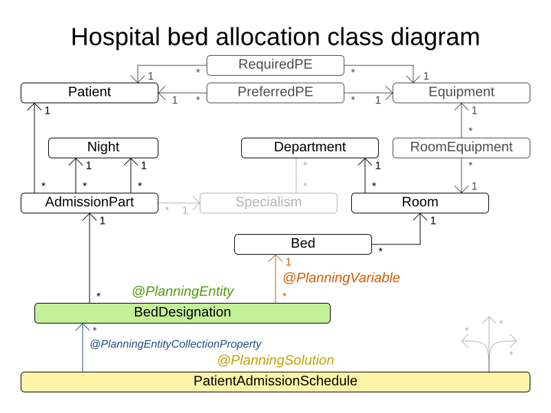
Schedule each exam into a period and into a room. Multiple exams can share the same room during the same period.
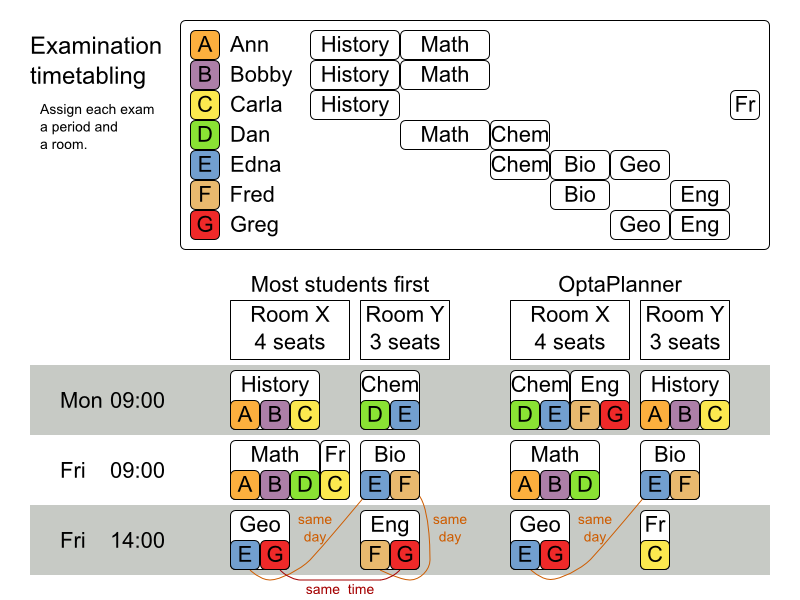
Hard constraints:
Exam conflict: 2 exams that share students must not occur in the same period.
Room capacity: A room's seating capacity must suffice at all times.
Period duration: A period's duration must suffice for all of its exams.
Period related hard constraints (specified per dataset):
Coincidence: 2 specified exams must use the same period (but possibly another room).
Exclusion: 2 specified exams must not use the same period.
After: A specified exam must occur in a period after another specified exam's period.
Room related hard constraints (specified per dataset):
Exclusive: 1 specified exam should not have to share its room with any other exam.
Soft constraints (each of which has a parametrized penalty):
The same student should not have 2 exams in a row.
The same student should not have 2 exams on the same day.
Period spread: 2 exams that share students should be a number of periods apart.
Mixed durations: 2 exams that share a room should not have different durations.
Front load: Large exams should be scheduled earlier in the schedule.
Period penalty (specified per dataset): Some periods have a penalty when used.
Room penalty (specified per dataset): Some rooms have a penalty when used.
It uses large test data sets of real-life universities.
The problem is defined by the International Timetabling Competition 2007 track 1. Geoffrey De Smet finished 4th in that competition with a very early version of Planner. Many improvements have been made since then.
exam_comp_set1 has  7883 students,  607 exams, 54 periods,  7 rooms,  12 period constraints and  0 room constraints with a search space of 10^1564.
exam_comp_set2 has 12484 students,  870 exams, 40 periods, 49 rooms,  12 period constraints and  2 room constraints with a search space of 10^2864.
exam_comp_set3 has 16365 students,  934 exams, 36 periods, 48 rooms, 168 period constraints and 15 room constraints with a search space of 10^3023.
exam_comp_set4 has  4421 students,  273 exams, 21 periods,  1 rooms,  40 period constraints and  0 room constraints with a search space of  10^360.
exam_comp_set5 has  8719 students, 1018 exams, 42 periods,  3 rooms,  27 period constraints and  0 room constraints with a search space of 10^2138.
exam_comp_set6 has  7909 students,  242 exams, 16 periods,  8 rooms,  22 period constraints and  0 room constraints with a search space of  10^509.
exam_comp_set7 has 13795 students, 1096 exams, 80 periods, 15 rooms,  28 period constraints and  0 room constraints with a search space of 10^3374.
exam_comp_set8 has 7718 students, 598 exams, 80 periods, 8 rooms, 20 period constraints and 1 room constraints with a search space of 10^1678.Below you can see the main examination domain classes:
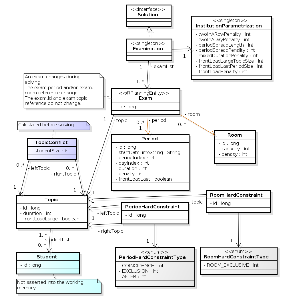
Notice that we've split up the exam concept into an Exam class and a
Topic class. The Exam instances change during solving (this is the
planning entity class), when their period or room property changes. The Topic,
Period and Room instances never change during solving (these are problem
facts, just like some other classes).
For each shift, assign a nurse to work that shift.
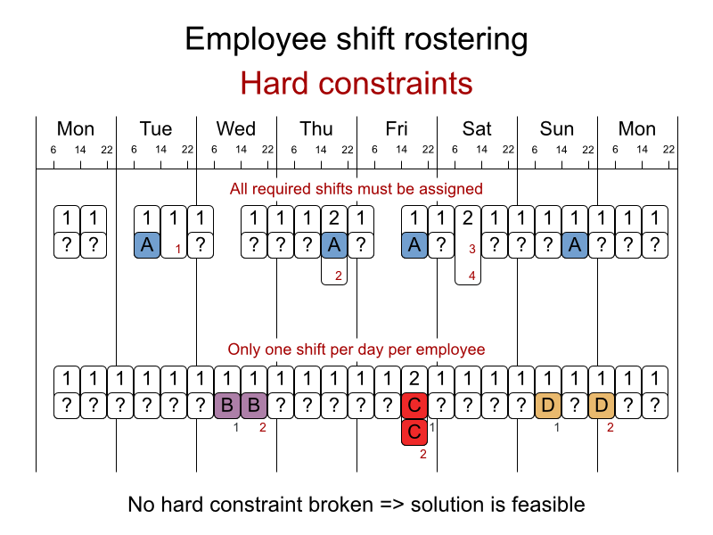
Hard constraints:
No unassigned shifts (build-in): Every shift need to be assigned to an employee.
Shift conflict: An employee can have only 1 shift per day.
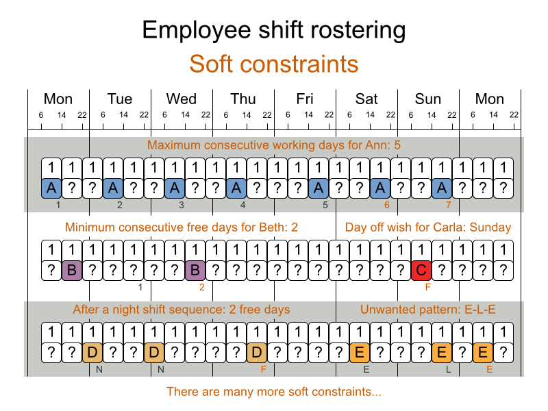
Soft constraints:
Contract obligations. The business frequently violates these, so they decided to define these as soft constraints instead of hard constraints.
Minimum and maximum assignments: Each employee needs to work more than x shifts and less than y shifts (depending on their contract).
Minimum and maximum consecutive working days: Each employee needs to work between x and y days in a row (depending on their contract).
Minimum and maximum consecutive free days: Each employee needs to be free between x and y days in a row (depending on their contract).
Minimum and maximum consecutive working weekends: Each employee needs to work between x and y weekends in a row (depending on their contract).
Complete weekends: Each employee needs to work every day in a weekend or not at all.
Identical shift types during weekend: Each weekend shift for the same weekend of the same employee must be the same shift type.
Unwanted patterns: A combination of unwanted shift types in a row. For example: a late shift followed by an early shift followed by a late shift.
Employee wishes:
Day on request: An employee wants to work on a specific day.
Day off request: An employee does not want to work on a specific day.
Shift on request: An employee wants to be assigned to a specific shift.
Shift off request: An employee does not want to be assigned to a specific shift.
Alternative skill: An employee assigned to a skill should have a proficiency in every skill required by that shift.
The problem is defined by the International Nurse Rostering Competition 2010.
There are 3 dataset types:
sprint: must be solved in seconds.
medium: must be solved in minutes.
long: must be solved in hours.
toy1          has 1 skills, 3 shiftTypes, 2 patterns, 1 contracts,  6 employees,  7 shiftDates,  35 shiftAssignments and   0 requests with a search space of   10^27.
toy2          has 1 skills, 3 shiftTypes, 3 patterns, 2 contracts, 20 employees, 28 shiftDates, 180 shiftAssignments and 140 requests with a search space of  10^234.

sprint01      has 1 skills, 4 shiftTypes, 3 patterns, 4 contracts, 10 employees, 28 shiftDates, 152 shiftAssignments and 150 requests with a search space of  10^152.
sprint02      has 1 skills, 4 shiftTypes, 3 patterns, 4 contracts, 10 employees, 28 shiftDates, 152 shiftAssignments and 150 requests with a search space of  10^152.
sprint03      has 1 skills, 4 shiftTypes, 3 patterns, 4 contracts, 10 employees, 28 shiftDates, 152 shiftAssignments and 150 requests with a search space of  10^152.
sprint04      has 1 skills, 4 shiftTypes, 3 patterns, 4 contracts, 10 employees, 28 shiftDates, 152 shiftAssignments and 150 requests with a search space of  10^152.
sprint05      has 1 skills, 4 shiftTypes, 3 patterns, 4 contracts, 10 employees, 28 shiftDates, 152 shiftAssignments and 150 requests with a search space of  10^152.
sprint06      has 1 skills, 4 shiftTypes, 3 patterns, 4 contracts, 10 employees, 28 shiftDates, 152 shiftAssignments and 150 requests with a search space of  10^152.
sprint07      has 1 skills, 4 shiftTypes, 3 patterns, 4 contracts, 10 employees, 28 shiftDates, 152 shiftAssignments and 150 requests with a search space of  10^152.
sprint08      has 1 skills, 4 shiftTypes, 3 patterns, 4 contracts, 10 employees, 28 shiftDates, 152 shiftAssignments and 150 requests with a search space of  10^152.
sprint09      has 1 skills, 4 shiftTypes, 3 patterns, 4 contracts, 10 employees, 28 shiftDates, 152 shiftAssignments and 150 requests with a search space of  10^152.
sprint10      has 1 skills, 4 shiftTypes, 3 patterns, 4 contracts, 10 employees, 28 shiftDates, 152 shiftAssignments and 150 requests with a search space of  10^152.
sprint_hint01 has 1 skills, 4 shiftTypes, 8 patterns, 3 contracts, 10 employees, 28 shiftDates, 152 shiftAssignments and 150 requests with a search space of  10^152.
sprint_hint02 has 1 skills, 4 shiftTypes, 0 patterns, 3 contracts, 10 employees, 28 shiftDates, 152 shiftAssignments and 150 requests with a search space of  10^152.
sprint_hint03 has 1 skills, 4 shiftTypes, 8 patterns, 3 contracts, 10 employees, 28 shiftDates, 152 shiftAssignments and 150 requests with a search space of  10^152.
sprint_late01 has 1 skills, 4 shiftTypes, 8 patterns, 3 contracts, 10 employees, 28 shiftDates, 152 shiftAssignments and 150 requests with a search space of  10^152.
sprint_late02 has 1 skills, 3 shiftTypes, 4 patterns, 3 contracts, 10 employees, 28 shiftDates, 144 shiftAssignments and 139 requests with a search space of  10^144.
sprint_late03 has 1 skills, 4 shiftTypes, 8 patterns, 3 contracts, 10 employees, 28 shiftDates, 160 shiftAssignments and 150 requests with a search space of  10^160.
sprint_late04 has 1 skills, 4 shiftTypes, 8 patterns, 3 contracts, 10 employees, 28 shiftDates, 160 shiftAssignments and 150 requests with a search space of  10^160.
sprint_late05 has 1 skills, 4 shiftTypes, 8 patterns, 3 contracts, 10 employees, 28 shiftDates, 152 shiftAssignments and 150 requests with a search space of  10^152.
sprint_late06 has 1 skills, 4 shiftTypes, 0 patterns, 3 contracts, 10 employees, 28 shiftDates, 152 shiftAssignments and 150 requests with a search space of  10^152.
sprint_late07 has 1 skills, 4 shiftTypes, 0 patterns, 3 contracts, 10 employees, 28 shiftDates, 152 shiftAssignments and 150 requests with a search space of  10^152.
sprint_late08 has 1 skills, 4 shiftTypes, 0 patterns, 3 contracts, 10 employees, 28 shiftDates, 152 shiftAssignments and   0 requests with a search space of  10^152.
sprint_late09 has 1 skills, 4 shiftTypes, 0 patterns, 3 contracts, 10 employees, 28 shiftDates, 152 shiftAssignments and   0 requests with a search space of  10^152.
sprint_late10 has 1 skills, 4 shiftTypes, 0 patterns, 3 contracts, 10 employees, 28 shiftDates, 152 shiftAssignments and 150 requests with a search space of  10^152.

medium01      has 1 skills, 4 shiftTypes, 0 patterns, 4 contracts, 31 employees, 28 shiftDates, 608 shiftAssignments and 403 requests with a search space of  10^906.
medium02      has 1 skills, 4 shiftTypes, 0 patterns, 4 contracts, 31 employees, 28 shiftDates, 608 shiftAssignments and 403 requests with a search space of  10^906.
medium03      has 1 skills, 4 shiftTypes, 0 patterns, 4 contracts, 31 employees, 28 shiftDates, 608 shiftAssignments and 403 requests with a search space of  10^906.
medium04      has 1 skills, 4 shiftTypes, 0 patterns, 4 contracts, 31 employees, 28 shiftDates, 608 shiftAssignments and 403 requests with a search space of  10^906.
medium05      has 1 skills, 4 shiftTypes, 0 patterns, 4 contracts, 31 employees, 28 shiftDates, 608 shiftAssignments and 403 requests with a search space of  10^906.
medium_hint01 has 1 skills, 4 shiftTypes, 7 patterns, 4 contracts, 30 employees, 28 shiftDates, 428 shiftAssignments and 390 requests with a search space of  10^632.
medium_hint02 has 1 skills, 4 shiftTypes, 7 patterns, 3 contracts, 30 employees, 28 shiftDates, 428 shiftAssignments and 390 requests with a search space of  10^632.
medium_hint03 has 1 skills, 4 shiftTypes, 7 patterns, 4 contracts, 30 employees, 28 shiftDates, 428 shiftAssignments and 390 requests with a search space of  10^632.
medium_late01 has 1 skills, 4 shiftTypes, 7 patterns, 4 contracts, 30 employees, 28 shiftDates, 424 shiftAssignments and 390 requests with a search space of  10^626.
medium_late02 has 1 skills, 4 shiftTypes, 7 patterns, 3 contracts, 30 employees, 28 shiftDates, 428 shiftAssignments and 390 requests with a search space of  10^632.
medium_late03 has 1 skills, 4 shiftTypes, 0 patterns, 4 contracts, 30 employees, 28 shiftDates, 428 shiftAssignments and 390 requests with a search space of  10^632.
medium_late04 has 1 skills, 4 shiftTypes, 7 patterns, 3 contracts, 30 employees, 28 shiftDates, 416 shiftAssignments and 390 requests with a search space of  10^614.
medium_late05 has 2 skills, 5 shiftTypes, 7 patterns, 4 contracts, 30 employees, 28 shiftDates, 452 shiftAssignments and 390 requests with a search space of  10^667.

long01        has 2 skills, 5 shiftTypes, 3 patterns, 3 contracts, 49 employees, 28 shiftDates, 740 shiftAssignments and 735 requests with a search space of 10^1250.
long02        has 2 skills, 5 shiftTypes, 3 patterns, 3 contracts, 49 employees, 28 shiftDates, 740 shiftAssignments and 735 requests with a search space of 10^1250.
long03        has 2 skills, 5 shiftTypes, 3 patterns, 3 contracts, 49 employees, 28 shiftDates, 740 shiftAssignments and 735 requests with a search space of 10^1250.
long04        has 2 skills, 5 shiftTypes, 3 patterns, 3 contracts, 49 employees, 28 shiftDates, 740 shiftAssignments and 735 requests with a search space of 10^1250.
long05        has 2 skills, 5 shiftTypes, 3 patterns, 3 contracts, 49 employees, 28 shiftDates, 740 shiftAssignments and 735 requests with a search space of 10^1250.
long_hint01   has 2 skills, 5 shiftTypes, 9 patterns, 3 contracts, 50 employees, 28 shiftDates, 740 shiftAssignments and   0 requests with a search space of 10^1257.
long_hint02   has 2 skills, 5 shiftTypes, 7 patterns, 3 contracts, 50 employees, 28 shiftDates, 740 shiftAssignments and   0 requests with a search space of 10^1257.
long_hint03   has 2 skills, 5 shiftTypes, 7 patterns, 3 contracts, 50 employees, 28 shiftDates, 740 shiftAssignments and   0 requests with a search space of 10^1257.
long_late01   has 2 skills, 5 shiftTypes, 9 patterns, 3 contracts, 50 employees, 28 shiftDates, 752 shiftAssignments and   0 requests with a search space of 10^1277.
long_late02   has 2 skills, 5 shiftTypes, 9 patterns, 4 contracts, 50 employees, 28 shiftDates, 752 shiftAssignments and   0 requests with a search space of 10^1277.
long_late03   has 2 skills, 5 shiftTypes, 9 patterns, 3 contracts, 50 employees, 28 shiftDates, 752 shiftAssignments and   0 requests with a search space of 10^1277.
long_late04   has 2 skills, 5 shiftTypes, 9 patterns, 4 contracts, 50 employees, 28 shiftDates, 752 shiftAssignments and   0 requests with a search space of 10^1277.
long_late05   has 2 skills, 5 shiftTypes, 9 patterns, 3 contracts, 50 employees, 28 shiftDates, 740 shiftAssignments and   0 requests with a search space of 10^1257.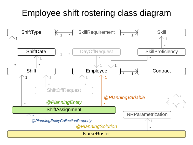
Schedule matches between n teams.
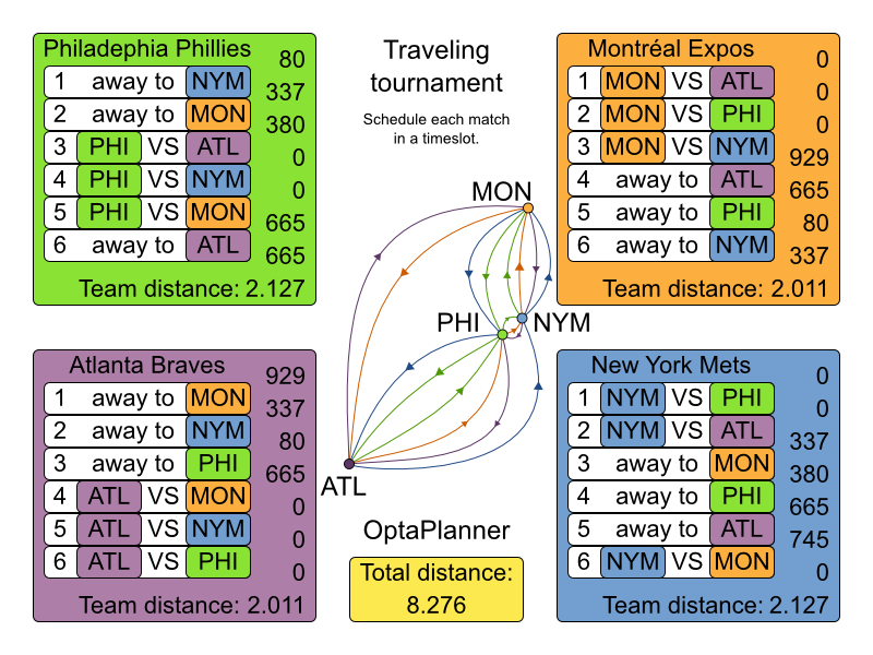
Hard constraints:
Each team plays twice against every other team: once home and once away.
Each team has exactly 1 match on each timeslot.
No team must have more than 3 consecutive home or 3 consecutive away matches.
No repeaters: no 2 consecutive matches of the same 2 opposing teams.
Soft constraints:
Minimize the total distance traveled by all teams.
The problem is defined on Michael Trick's website (which contains the world records too).
1-nl04     has  6 days,  4 teams and   12 matches with a search space of    10^9.
1-nl06     has 10 days,  6 teams and   30 matches with a search space of   10^30.
1-nl08     has 14 days,  8 teams and   56 matches with a search space of   10^64.
1-nl10     has 18 days, 10 teams and   90 matches with a search space of  10^112.
1-nl12     has 22 days, 12 teams and  132 matches with a search space of  10^177.
1-nl14     has 26 days, 14 teams and  182 matches with a search space of  10^257.
1-nl16     has 30 days, 16 teams and  240 matches with a search space of  10^354.
2-bra24    has 46 days, 24 teams and  552 matches with a search space of  10^917.
3-nfl16    has 30 days, 16 teams and  240 matches with a search space of  10^354.
3-nfl18    has 34 days, 18 teams and  306 matches with a search space of  10^468.
3-nfl20    has 38 days, 20 teams and  380 matches with a search space of  10^600.
3-nfl22    has 42 days, 22 teams and  462 matches with a search space of  10^749.
3-nfl24    has 46 days, 24 teams and  552 matches with a search space of  10^917.
3-nfl26    has 50 days, 26 teams and  650 matches with a search space of 10^1104.
3-nfl28    has 54 days, 28 teams and  756 matches with a search space of 10^1309.
3-nfl30    has 58 days, 30 teams and  870 matches with a search space of 10^1534.
3-nfl32    has 62 days, 32 teams and  992 matches with a search space of 10^1778.
4-super04  has  6 days,  4 teams and   12 matches with a search space of    10^9.
4-super06  has 10 days,  6 teams and   30 matches with a search space of   10^30.
4-super08  has 14 days,  8 teams and   56 matches with a search space of   10^64.
4-super10  has 18 days, 10 teams and   90 matches with a search space of  10^112.
4-super12  has 22 days, 12 teams and  132 matches with a search space of  10^177.
4-super14  has 26 days, 14 teams and  182 matches with a search space of  10^257.
5-galaxy04 has  6 days,  4 teams and   12 matches with a search space of    10^9.
5-galaxy06 has 10 days,  6 teams and   30 matches with a search space of   10^30.
5-galaxy08 has 14 days,  8 teams and   56 matches with a search space of   10^64.
5-galaxy10 has 18 days, 10 teams and   90 matches with a search space of  10^112.
5-galaxy12 has 22 days, 12 teams and  132 matches with a search space of  10^177.
5-galaxy14 has 26 days, 14 teams and  182 matches with a search space of  10^257.
5-galaxy16 has 30 days, 16 teams and  240 matches with a search space of  10^354.
5-galaxy18 has 34 days, 18 teams and  306 matches with a search space of  10^468.
5-galaxy20 has 38 days, 20 teams and  380 matches with a search space of  10^600.
5-galaxy22 has 42 days, 22 teams and  462 matches with a search space of  10^749.
5-galaxy24 has 46 days, 24 teams and  552 matches with a search space of  10^917.
5-galaxy26 has 50 days, 26 teams and  650 matches with a search space of 10^1104.
5-galaxy28 has 54 days, 28 teams and  756 matches with a search space of 10^1309.
5-galaxy30 has 58 days, 30 teams and  870 matches with a search space of 10^1534.
5-galaxy32 has 62 days, 32 teams and  992 matches with a search space of 10^1778.
5-galaxy34 has 66 days, 34 teams and 1122 matches with a search space of 10^2041.
5-galaxy36 has 70 days, 36 teams and 1260 matches with a search space of 10^2324.
5-galaxy38 has 74 days, 38 teams and 1406 matches with a search space of 10^2628.
5-galaxy40 has 78 days, 40 teams and 1560 matches with a search space of 10^2951.Schedule all tasks in time and on a machine to minimize power cost. Power prices differs in time. This is a form of job shop scheduling.
Hard constraints:
Start time limits: each task must start between its earliest start and latest start limit.
Maximum capacity: the maximum capacity for each resource for each machine must not be exceeded.
Startup and shutdown: each machine must be active in the periods during which it has assigned tasks. Between tasks it is allowed to be idle to avoid startup and shutdown costs.
Medium constraints:
Power cost: minimize the total power cost of the whole schedule.
Machine power cost: Each active or idle machine consumes power, which infers a power cost (depending on the power price during that time).
Task power cost: Each task consumes power too, which infers a power cost (depending on the power price during its time).
Machine startup and shutdown cost: Every time a machine starts up or shuts down, an extra cost is inflicted.
Soft constraints (addendum to the original problem definition):
Start early: prefer starting a task sooner rather than later.
The problem is defined by the ICON challenge.
sample01   has 3 resources,   2 machines, 288 periods and   25 tasks with a search space of    10^53.
sample02   has 3 resources,   2 machines, 288 periods and   50 tasks with a search space of   10^114.
sample03   has 3 resources,   2 machines, 288 periods and  100 tasks with a search space of   10^226.
sample04   has 3 resources,   5 machines, 288 periods and  100 tasks with a search space of   10^266.
sample05   has 3 resources,   2 machines, 288 periods and  250 tasks with a search space of   10^584.
sample06   has 3 resources,   5 machines, 288 periods and  250 tasks with a search space of   10^673.
sample07   has 3 resources,   2 machines, 288 periods and 1000 tasks with a search space of  10^2388.
sample08   has 3 resources,   5 machines, 288 periods and 1000 tasks with a search space of  10^2748.
sample09   has 4 resources,  20 machines, 288 periods and 2000 tasks with a search space of  10^6668.
instance00 has 1 resources,  10 machines, 288 periods and  200 tasks with a search space of   10^595.
instance01 has 1 resources,  10 machines, 288 periods and  200 tasks with a search space of   10^599.
instance02 has 1 resources,  10 machines, 288 periods and  200 tasks with a search space of   10^599.
instance03 has 1 resources,  10 machines, 288 periods and  200 tasks with a search space of   10^591.
instance04 has 1 resources,  10 machines, 288 periods and  200 tasks with a search space of   10^590.
instance05 has 2 resources,  25 machines, 288 periods and  200 tasks with a search space of   10^667.
instance06 has 2 resources,  25 machines, 288 periods and  200 tasks with a search space of   10^660.
instance07 has 2 resources,  25 machines, 288 periods and  200 tasks with a search space of   10^662.
instance08 has 2 resources,  25 machines, 288 periods and  200 tasks with a search space of   10^651.
instance09 has 2 resources,  25 machines, 288 periods and  200 tasks with a search space of   10^659.
instance10 has 2 resources,  20 machines, 288 periods and  500 tasks with a search space of  10^1657.
instance11 has 2 resources,  20 machines, 288 periods and  500 tasks with a search space of  10^1644.
instance12 has 2 resources,  20 machines, 288 periods and  500 tasks with a search space of  10^1637.
instance13 has 2 resources,  20 machines, 288 periods and  500 tasks with a search space of  10^1659.
instance14 has 2 resources,  20 machines, 288 periods and  500 tasks with a search space of  10^1643.
instance15 has 3 resources,  40 machines, 288 periods and  500 tasks with a search space of  10^1782.
instance16 has 3 resources,  40 machines, 288 periods and  500 tasks with a search space of  10^1778.
instance17 has 3 resources,  40 machines, 288 periods and  500 tasks with a search space of  10^1764.
instance18 has 3 resources,  40 machines, 288 periods and  500 tasks with a search space of  10^1769.
instance19 has 3 resources,  40 machines, 288 periods and  500 tasks with a search space of  10^1778.
instance20 has 3 resources,  50 machines, 288 periods and 1000 tasks with a search space of  10^3689.
instance21 has 3 resources,  50 machines, 288 periods and 1000 tasks with a search space of  10^3678.
instance22 has 3 resources,  50 machines, 288 periods and 1000 tasks with a search space of  10^3706.
instance23 has 3 resources,  50 machines, 288 periods and 1000 tasks with a search space of  10^3676.
instance24 has 3 resources,  50 machines, 288 periods and 1000 tasks with a search space of  10^3681.
instance25 has 3 resources,  60 machines, 288 periods and 1000 tasks with a search space of  10^3774.
instance26 has 3 resources,  60 machines, 288 periods and 1000 tasks with a search space of  10^3737.
instance27 has 3 resources,  60 machines, 288 periods and 1000 tasks with a search space of  10^3744.
instance28 has 3 resources,  60 machines, 288 periods and 1000 tasks with a search space of  10^3731.
instance29 has 3 resources,  60 machines, 288 periods and 1000 tasks with a search space of  10^3746.
instance30 has 4 resources,  70 machines, 288 periods and 2000 tasks with a search space of  10^7718.
instance31 has 4 resources,  70 machines, 288 periods and 2000 tasks with a search space of  10^7740.
instance32 has 4 resources,  70 machines, 288 periods and 2000 tasks with a search space of  10^7686.
instance33 has 4 resources,  70 machines, 288 periods and 2000 tasks with a search space of  10^7672.
instance34 has 4 resources,  70 machines, 288 periods and 2000 tasks with a search space of  10^7695.
instance35 has 4 resources,  80 machines, 288 periods and 2000 tasks with a search space of  10^7807.
instance36 has 4 resources,  80 machines, 288 periods and 2000 tasks with a search space of  10^7814.
instance37 has 4 resources,  80 machines, 288 periods and 2000 tasks with a search space of  10^7764.
instance38 has 4 resources,  80 machines, 288 periods and 2000 tasks with a search space of  10^7736.
instance39 has 4 resources,  80 machines, 288 periods and 2000 tasks with a search space of  10^7783.
instance40 has 4 resources,  90 machines, 288 periods and 4000 tasks with a search space of 10^15976.
instance41 has 4 resources,  90 machines, 288 periods and 4000 tasks with a search space of 10^15935.
instance42 has 4 resources,  90 machines, 288 periods and 4000 tasks with a search space of 10^15887.
instance43 has 4 resources,  90 machines, 288 periods and 4000 tasks with a search space of 10^15896.
instance44 has 4 resources,  90 machines, 288 periods and 4000 tasks with a search space of 10^15885.
instance45 has 4 resources, 100 machines, 288 periods and 5000 tasks with a search space of 10^20173.
instance46 has 4 resources, 100 machines, 288 periods and 5000 tasks with a search space of 10^20132.
instance47 has 4 resources, 100 machines, 288 periods and 5000 tasks with a search space of 10^20126.
instance48 has 4 resources, 100 machines, 288 periods and 5000 tasks with a search space of 10^20110.
instance49 has 4 resources, 100 machines, 288 periods and 5000 tasks with a search space of 10^20078.Solving a planning problem with Planner consists out of 5 steps:
Model your planning problem as a class that implements the interface
Solution, for example the classNQueens.Configure a
Solver, for example a First Fit and Tabu Search solver for anyNQueensinstance.Load a problem data set from your data layer, for example a 4 Queens instance. That is the planning problem.
Solve it with
Solver.solve(planningProblem).Get the best solution found by the
SolverwithSolver.getBestSolution().
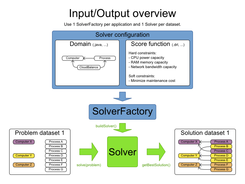
Build a Solver instance with the SolverFactory. Configure it with a
solver configuration XML file, provided as a classpath resource (as definied by
ClassLoader.getResource()):
       SolverFactory solverFactory = SolverFactory.createFromXmlResource(
               "org/optaplanner/examples/nqueens/solver/nqueensSolverConfig.xml");
       Solver solver = solverFactory.buildSolver();
In a typical project (following the Maven directory structure), that solverConfig XML file would be located
at
$PROJECT_DIR/src/main/resources/org/optaplanner/examples/nqueens/solver/nqueensSolverConfig.xml.
On some environments (OSGi, JBoss modules, ...), classpath resources in your jars might not be
available in by default to the classes in optaplanner's jars.
Alternatively, a SolverFactory can be created from a File, an
InputStream or a Reader with methods such as
SolverFactory.createFromXmlFile(). However, for portability reasons, a classpath resource is
recommended.
A solver configuration file looks like this:
<?xml version="1.0" encoding="UTF-8"?>
<solver>
  <!-- Define the model -->
  <solutionClass>org.optaplanner.examples.nqueens.domain.NQueens</solutionClass>
  <entityClass>org.optaplanner.examples.nqueens.domain.Queen</entityClass>

  <!-- Define the score function -->
  <scoreDirectorFactory>
    <scoreDefinitionType>SIMPLE</scoreDefinitionType>
    <scoreDrl>org/optaplanner/examples/nqueens/solver/nQueensScoreRules.drl</scoreDrl>
  </scoreDirectorFactory>

  <!-- Configure the optimization algorithm(s) -->
  <termination>
    ...
  </termination>
  <constructionHeuristic>
    ...
  </constructionHeuristic>
  <localSearch>
    ...
  </localSearch>
</solver>
Notice the three parts in it:
Define the model
Define the score function
Configure the optimization algorithm(s)
These various parts of a configuration are explained further in this manual.
Planner makes it relatively easy to switch optimization algorithm(s) just by changing
the configuration. There is even a Benchmarker utility which allows you to play out
different configurations against each other and report the most appropriate configuration for your use
case.
A solver configuration can also be configured with the SolverConfig API. This is
especially useful to change some values dynamically at runtime. For example, to change the running time based on
user input, before building the Solver:
        SolverFactory solverFactory = SolverFactory.createFromXmlResource(
                "org/optaplanner/examples/nqueens/solver/nqueensSolverConfig.xml");

        TerminationConfig terminationConfig = new TerminationConfig();
        terminationConfig.setMinutesSpentLimit(userInput);
        solverFactory.getSolverConfig().setTerminationConfig(terminationConfig);

        Solver solver = solverFactory.buildSolver();
Every element in the solver configuration XML is available as a *Config class or a
property on a *Config class in the package namespace
org.optaplanner.core.config. These *Config classes are the Java
representation of the XML format and they also provide the user-friendly way to assemble the runtime components
(of the package namespace org.optaplanner.core.impl) into an efficient
Solver.
Look at a dataset of your planning problem. You will recognize domain classes in there, each of which can be categorized as one of the following:
A unrelated class: not used by any of the score constraints. From a planning standpoint, this data is obsolete.
A problem fact class: used by the score constraints, but does NOT change during planning (as long as the problem stays the same). For example:
Bed,Room,Shift,Employee,Topic,Period, ... All the properties of a problem fact class are problem properties.A planning entity class: used by the score constraints and changes during planning. For example:
BedDesignation,ShiftAssignment,Exam, ... The properties that change during planning are planning variables. The other properties are problem properties.
Ask yourself: What class changes during planning? Which class has variables
that I want the Solver to change for me? That class is a planning entity. Most use
cases have only one planning entity class. Most use cases also have only one planning variable per planning entity
class.
Note
In real-time planning, even though the problem itself changes, problem facts do not really change during planning, instead they change between planning (because the Solver temporarily stops to apply the problem fact changes).
A good model can greatly improve the success of your planning implementation. Follow these guidelines to design a good model:
In a many to one relationship, it is normally the many side that is the planning entity class. The property referencing the other side is then the planning variable. For example in employee rostering: the planning entity class is
ShiftAssignment, notEmployee, and the planning variable isShiftAssignment.getEmployee()because oneEmployeehas multipleShiftAssignments but oneShiftAssignmenthas only oneEmployee.A planning entity class should have at least one problem property. A planning entity class with only planning variables can normally be simplified by converting one of those planning variables into a problem property. That heavily decreases the search space size. For example in employee rostering: the
ShiftAssignment'sgetShift()is a problem property and thegetEmployee()is a planning variable. If both were a planning variable, solving it would be far less efficient.A surrogate ID does not suffice as the required minimum of one problem property. It needs to be understandable by the business. A business key does suffice. This prevents an unassigned entity from being nameless (unidentifiable by the business).
This way, there is no need to add a hard constraint to assure that two planning entities are different: they are already different due to their problem properties.
In some cases, multiple planning entities have the same problem property. In such cases, it can be useful to create an extra problem property to distinguish them. For example in employee rostering:
ShiftAssignmenthas besides the problem propertyShiftalso the problem propertyindexInShift.
The number of planning entities is recommended to be fixed during planning. When unsure of which property should be a planning variable and which should be a problem property, choose it so the number of planning entities is fixed. For example in employee rostering: if the planning entity class would have been
EmployeeAssignmentwith a problem propertygetEmployee()and a planning variablegetShift(), than it is impossible to accurately predict how manyEmployeeAssignmentinstances to make perEmployee.
For inspiration, take a look at how the examples modeled their domain:
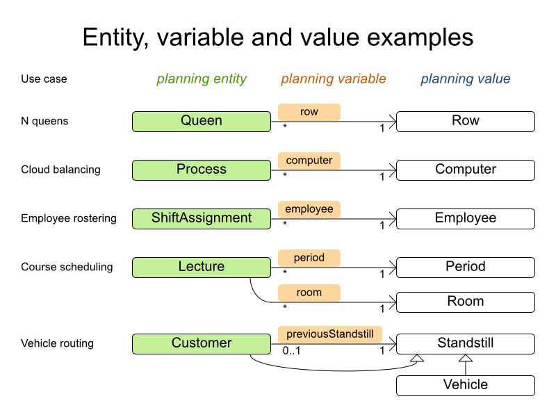
Note
Vehicle routing is special, because it uses a chained planning variable.
In Planner all problems facts and planning entities are plain old JavaBeans (POJOs). You can load them from a database, an XML file, a data repository, a noSQL cloud, ... (see Integration).
Planner needs to be told which classes in your domain model are planning entities, which properties are planning variables, etc. There are several ways to deliver this information:
Add class annotations and JavaBean property annotations on the domain model. The property annotations must be the getter method, not on the setter method. This is the recommended manner.
Add class annotations and field annotations on the domain model.
No annotations: externalize the domain configuration in an XML file. This is not yet supported.
This manual focusses on the first manner, but every features supports all 3 manners, even if it's not explicilty mentioned.
A problem fact is any JavaBean (POJO) with getters that does not change during planning. Implementing the
interface Serializable is recommended (but not required). For example in n queens, the columns
and rows are problem facts:
public class Column implements Serializable {

    private int index;

    // ... getters
}
public class Row implements Serializable {
private int index;
// ... getters
}A problem fact can reference other problem facts of course:
public class Course implements Serializable {

    private String code;

    private Teacher teacher; // Other problem fact
    private int lectureSize;
    private int minWorkingDaySize;

    private List<Curriculum> curriculumList; // Other problem facts
    private int studentSize;

    // ... getters
}
A problem fact class does not require any Planner specific code. For example, you can reuse your domain classes, which might have JPA annotations.
Note
Generally, better designed domain classes lead to simpler and more efficient score constraints. Therefore,
when dealing with a messy (denormalized) legacy system, it can sometimes be worthwhile to convert the messy
domain model into a Planner specific model first. For example: if your domain model has two
Teacher instances for the same teacher that teaches at two different departments, it is
harder to write a correct score constraint that constrains a teacher's spare time on the original model than on
an adjusted model.
Alternatively, you can sometimes also introduce a cached problem fact to enrich the domain model for planning only.
A planning entity is a JavaBean (POJO) that changes during solving, for example a Queen
that changes to another row. A planning problem has multiple planning entities, for example for a single n
queens problem, each Queen is a planning entity. But there is usually only one planning
entity class, for example the Queen class.
A planning entity class needs to be annotated with the @PlanningEntity
annotation.
Each planning entity class has one or more planning variables. It should also have
one or more defining properties. For example in n queens, a Queen is
defined by its Column and has a planning variable Row. This means that a
Queen's column never changes during solving, while its row does change.
@PlanningEntity
public class Queen {

    private Column column;

    // Planning variables: changes during planning, between score calculations.
    private Row row;

    // ... getters and setters
}
A planning entity class can have multiple planning variables. For example, a Lecture is
defined by its Course and its index in that course (because one course has multiple
lectures). Each Lecture needs to be scheduled into a Period and a
Room so it has two planning variables (period and room). For example: the course Mathematics
has eight lectures per week, of which the first lecture is Monday morning at 08:00 in room 212.
@PlanningEntity
public class Lecture {

    private Course course;
    private int lectureIndexInCourse;

    // Planning variables: changes during planning, between score calculations.
    private Period period;
    private Room room;

    // ...
}
The solver configuration also needs to be made aware of each planning entity class:
<solver>
  ...
  <entityClass>org.optaplanner.examples.nqueens.domain.Queen</entityClass>
  ...
</solver>
Some uses cases have multiple planning entity classes. For example: route freight and trains into railway network arcs, where each freight can use multiple trains over its journey and each train can carry multiple freights per arc. Having multiple planning entity classes directly raises the implementation complexity of your use case.
Note
Do not create unnecessary planning entity classes. This leads to difficult
Move implementations and slower score calculation.
For example, do not create a planning entity class to hold the total free time of a teacher, which needs
to be kept up to date as the Lecture planning entities change. Instead, calculate the free
time in the score constraints and put the result per teacher into a logically inserted score object.
If historic data needs to be considered too, then create problem fact to hold the total of the historic assignments up to, but not including, the planning window (so it doesn't change when a planning entity changes) and let the score constraints take it into account.
Some optimization algorithms work more efficiently if they have an estimation of which planning entities are more difficult to plan. For example: in bin packing bigger items are harder to fit, in course scheduling lectures with more students are more difficult to schedule and in n queens the middle queens are more difficult to fit on the board.
Therefore, you can set a difficultyComparatorClass to the
@PlanningEntity annotation:
@PlanningEntity(difficultyComparatorClass = CloudProcessDifficultyComparator.class)
public class CloudProcess {
    // ...
}
public class CloudProcessDifficultyComparator implements Comparator<CloudProcess> {
public int compare(CloudProcess a, CloudProcess b) {
return new CompareToBuilder()
.append(a.getRequiredMultiplicand(), b.getRequiredMultiplicand())
.append(a.getId(), b.getId())
.toComparison();
}
}Alternatively, you can also set a difficultyWeightFactoryClass to the
@PlanningEntity annotation, so you have access to the rest of the problem facts from the
Solution too:
@PlanningEntity(difficultyWeightFactoryClass = QueenDifficultyWeightFactory.class)
public class Queen {
// ...
}See sorted selection for more information.
Important
Difficulty should be implemented ascending: easy entities are lower, difficult entities are higher. For example in bin packing: small item < medium item < big item.
Even though some algorithms start with the more difficult entities first, they just reverse the ordering.
None of the current planning variable states should be used to compare planning entity
difficult. During Construction Heuristics, those variables are likely to be null
anyway. For example, a Queen's row variable should not be used.
A planning variable is a JavaBean property (so a getter and setter) on a planning entity. It points to a
planning value, which changes during planning. For example, a Queen's row
property is a planning variable. Note that even though a Queen's row
property changes to another Row during planning, no Row instance itself is
changed.
A planning variable getter needs to be annotated with the @PlanningVariable annotation,
which needs a non-empty valueRangeProviderRefs property.
@PlanningEntity
public class Queen {
...
private Row row;
@PlanningVariable(valueRangeProviderRefs = {"rowRange"})
public Row getRow() {
return row;
}
public void setRow(Row row) {
this.row = row;
}
}The valueRangeProviderRefs property defines what are the possible planning values for
this planning variable. It references one or more @ValueRangeProvider
id's.
Annotating the field instead of the property works too:
@PlanningEntity
public class Queen {
...
@PlanningVariable(valueRangeProviderRefs = {"rowRange"})
private Row row;
}By default, an initialized planning variable cannot be null, so an initialized solution
will never use null for any of its planning variables. In an over-constrained use case, this
can be counterproductive. For example: in task assignment with too many tasks for the workforce, we would rather
leave low priority tasks unassigned instead of assigning them to an overloaded worker.
To allow an initialized planning variable to be null, set nullable
to true:
@PlanningVariable(..., nullable = true)
public Worker getWorker() {
return worker;
}Important
Planner will automatically add the value null to the value range. There is no need to
add null in a collection used by a ValueRangeProvider.
Note
Using a nullable planning variable implies that your score calculation is responsible for punishing (or even rewarding) variables with a null value.
Repeated planning (especially real-time planning) does not mix well with a nullable planning variable: every
time the Solver starts or a problem fact change is made, the Construction
Heuristics will try to initialize all the null variables again, which can be a huge
waste of time. One way to deal with this, is to change when a planning entity should be reinitialized with an
reinitializeVariableEntityFilter:
@PlanningVariable(..., nullable = true, reinitializeVariableEntityFilter = ReinitializeTaskFilter.class)
public Worker getWorker() {
return worker;
}A planning variable is considered initialized if its value is not null or if the
variable is nullable. So a nullable variable is always considered initialized, even when a
custom reinitializeVariableEntityFilter triggers a reinitialization during construction
heuristics.
A planning entity is initialized if all of its planning variables are initialized.
A Solution is initialized if all of its planning entities are initialized.
A planning value is a possible value for a planning variable. Usually, a planning value is a problem fact,
but it can also be any object, for example a double. It can even be another planning entity
or even a interface implemented by both a planning entity and a problem fact.
A planning value range is the set of possible planning values for a planning variable. This set can be a
countable (for example row 1, 2, 3 or
4) or uncountable (for example any double between 0.0
and 1.0).
The value range of a planning variable is defined with the @ValueRangeProvider
annotation. A @ValueRangeProvider annotation always has a property id,
which is referenced by the @PlanningVariable's property
valueRangeProviderRefs.
This annotation can be located on 2 types of methods:
On the Solution: All planning entities share the same value range.
On the planning entity: The value range differs per planning entity. This is less common.
The return type of that method can be 2 types:
Collection: The value range is defined by aCollection(usually aList) of it's possible values.ValueRange: The value range is defined by its bounds. This is less common.
All instances of the same planning entity class share the same set of possible planning values for that planning variable. This is the most common way to configure a value range.
The Solution implementation has method which returns a Collection
(or a ValueRange). Any value from that Collection is a possible planning
value for this planning variable.
@PlanningVariable(valueRangeProviderRefs = {"rowRange"})
public Row getRow() {
return row;
}@PlanningSolution
public class NQueens implements Solution<SimpleScore> {
// ...
@ValueRangeProvider(id = "rowRange")
public List<Row> getRowList() {
return rowList;
}
}Important
That Collection (or ValueRange) must not contain the value
null, not even for a nullable planning
variable.
Annotating the field instead of the property works too:
@PlanningSolution
public class NQueens implements Solution<SimpleScore> {
...
@ValueRangeProvider(id = "rowRange")
private List<Row> rowList;
}Each planning entity has its own value range (a set of possible planning values) for the planning variable. For example, if a teacher can never teach in a room that does not belong to his department, lectures of that teacher can limit their room value range to the rooms of his department.
@PlanningVariable(valueRangeProviderRefs = {"departmentRoomRange"})
public Room getRoom() {
return room;
}
@ValueRangeProvider(id = "departmentRoomRange")
public List<Room> getPossibleRoomList() {
return getCourse().getTeacher().getDepartment().getRoomList();
}Never use this to enforce a soft constraint (or even a hard constraint when the problem might not have a feasible solution). For example: Unless there is no other way, a teacher can not teach in a room that does not belong to his department. In this case, the teacher should not be limited in his room value range (because sometimes there is no other way).
Note
By limiting the value range specifically of 1 planning entity, you are effectively creating a built-in hard constraint. This can be a very good thing, as the number of possible solutions is severely lowered. But this can also be a bad thing because it takes away the freedom of the optimization algorithms to temporarily break that constraint in order to escape from a local optimum.
A planning entity should not use other planning entities to determinate its value range. That would only try to make it solve the planning problem itself and interfere with the optimization algorithms.
Every entity has its own List instance, except if multiple entity have the same value
range. For example, if teacher A and B belong to the same department, they use the same
List<Room> instance. Furthermore, each List contains a subset of
the same set of planning value instances. For example, if department A and B can both use room X, then their
List<Room> instances contain the same Room instance.
Note
A ValueRangeProvider on the planning entity consumes more memory than
ValueRangeProvider on the Solution and disables certain automatic performance
optimizations.
Warning
A ValueRangeProvider on the planning entity is not (yet) compatible with a chained variable.
Instead of a Collection, you can also return a ValueRange or
CountableValueRange, build by the ValueRangeFactory:
@ValueRangeProvider(id = "delayRange")
public CountableValueRange<Integer> getDelayRange() {
return ValueRangeFactory.createIntValueRange(0, 5000);
}A ValueRange uses far less memory, because it only holds the bounds. In the example
above, a Collection would need to hold all 5000 ints, instead of just
the 2 bounds.
Furthermore, an incrementUnit can be specified, for example if you have to buy stocks
in units of 200 pieces:
@ValueRangeProvider(id = "stockAmountRange")
public CountableValueRange<Integer> getStockAmountRange() {
// Range: 0, 200, 400, 600, ..., 9999600, 9999800, 10000000
return ValueRangeFactory.createIntValueRange(0, 10000000, 200);
}Note
Return CountableValueRange instead of ValueRange whenever
possible (so Planner knows it's countable).
The ValueRangeFactory has creation methods for several value class types:
int: A 32bit integer range.long: A 64bit integer range.double: A 64bit floating point range which only supports random selection (because it does not implementCountableValueRange).BigDecimal: A decimal point range. By default, the increment unit is the lowest non-zero value in the scale of the bounds.
Value range providers can be combined, for example:
@PlanningVariable(valueRangeProviderRefs = {"companyCarRange", "personalCarRange"})
public Car getCar() {
return car;
} @ValueRangeProvider(id = "companyCarRange")
public List<CompanyCar> getCompanyCarList() {
return companyCarList;
}
@ValueRangeProvider(id = "personalCarRange")
public List<PersonalCar> getPersonalCarList() {
return personalCarList;
}Some optimization algorithms work more efficiently if they have an estimation of which planning values are stronger, which means they are more likely to satisfy a planning entity. For example: in bin packing bigger containers are more likely to fit an item and in course scheduling bigger rooms are less likely to break the student capacity constraint.
Therefore, you can set a strengthComparatorClass to the
@PlanningVariable annotation:
@PlanningVariable(..., strengthComparatorClass = CloudComputerStrengthComparator.class)
public CloudComputer getComputer() {
// ...
}public class CloudComputerStrengthComparator implements Comparator<CloudComputer> {
public int compare(CloudComputer a, CloudComputer b) {
return new CompareToBuilder()
.append(a.getMultiplicand(), b.getMultiplicand())
.append(b.getCost(), a.getCost()) // Descending (but this is debatable)
.append(a.getId(), b.getId())
.toComparison();
}
}Note
If you have multiple planning value classes in the same value range, the
strengthComparatorClass needs to implement a Comparator of a common
superclass (for example Comparator<Object>) and be able to handle comparing instances
of those different classes.
Alternatively, you can also set a strengthWeightFactoryClass to the
@PlanningVariable annotation, so you have access to the rest of the problem facts from the
solution too:
@PlanningVariable(..., strengthWeightFactoryClass = RowStrengthWeightFactory.class)
public Row getRow() {
// ...
}See sorted selection for more information.
Important
Strength should be implemented ascending: weaker values are lower, stronger values are higher. For example in bin packing: small container < medium container < big container.
None of the current planning variable state in any of the planning entities should be used to
compare planning values. During construction heuristics, those variables are likely to be
null anyway. For example, none of the row variables of any
Queen may be used to determine the strength of a Row.
Some use cases, such as TSP and Vehicle Routing, require chaining. This means the planning entities point to each other and form a chain. By modeling the problem as a set of chains (instead of a set of trees/loops), the search space is heavily reduced.
A planning variable that is chained either:
Directly points to a problem fact (or planning entity), which is called an anchor.
Points to another planning entity with the same planning variable, which recursively points to an anchor.
Here are some example of valid and invalid chains:
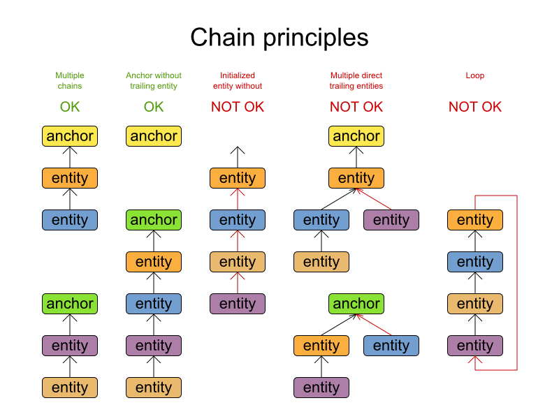
Every initialized planning entity is part of an open-ended chain that begins from an anchor. A valid model means that:
A chain is never a loop. The tail is always open.
Every chain always has exactly 1 anchor. The anchor is a problem fact, never a planning entity.
A chain is never a tree, it is always a line. Every anchor or planning entity has at most 1 trailing planning entity.
Every initialized planning entity is part of a chain.
An anchor with no planning entities pointing to it, is also considered a chain.
Warning
A planning problem instance given to the Solver must be valid.
Note
If your constraints dictate a closed chain, model it as an open-ended chain (which is easier to persist in a database) and implement a score constraint for the last entity back to the anchor.
The optimization algorithms and built-in Move's do chain correction to guarantee that
the model stays valid:
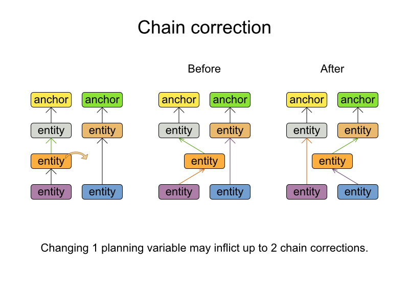
Warning
A custom Move implementation must leave the model in a valid state.
For example, in TSP the anchor is a Domicile (in vehicle routing it is
Vehicle):
public class Domicile ... implements Standstill {
...
public City getCity() {...}
}The anchor (which is a problem fact) and the planning entity implement a common interface, for example
TSP's Standstill:
public interface Standstill {
City getCity();
}That interface is the return type of the planning variable. Furthermore, the planning variable is chained.
For example TSP's Visit (in vehicle routing it is Customer):
@PlanningEntity
public class Visit ... implements Standstill {
...
public City getCity() {...}
@PlanningVariable(graphType = PlanningVariableGraphType.CHAINED, valueRangeProviderRefs = {"domicileRange", "visitRange"})
public Standstill getPreviousStandstill() {
return previousStandstill;
}
public void setPreviousStandstill(Standstill previousStandstill) {
this.previousStandstill = previousStandstill;
}
}Notice how 2 value range providers are usually combined:
The value range provider which holds the anchors, for example
domicileList.The value range provider which holds the initialized planning entities, for example
visitList.
A shadow variable is a variable whose correct value can be deduced from the state of the genuine planning variables. Even though such a variable violates the principle of normalization by definition, in some use cases it can be very practical to use a shadow variable, especially to express the constraints more naturally. For example in vehicle routing with time windows: the arrival time at a customer for a vehicle can be calculated based on the previously visited customers of that vehicle (and the known travel times between 2 locations).
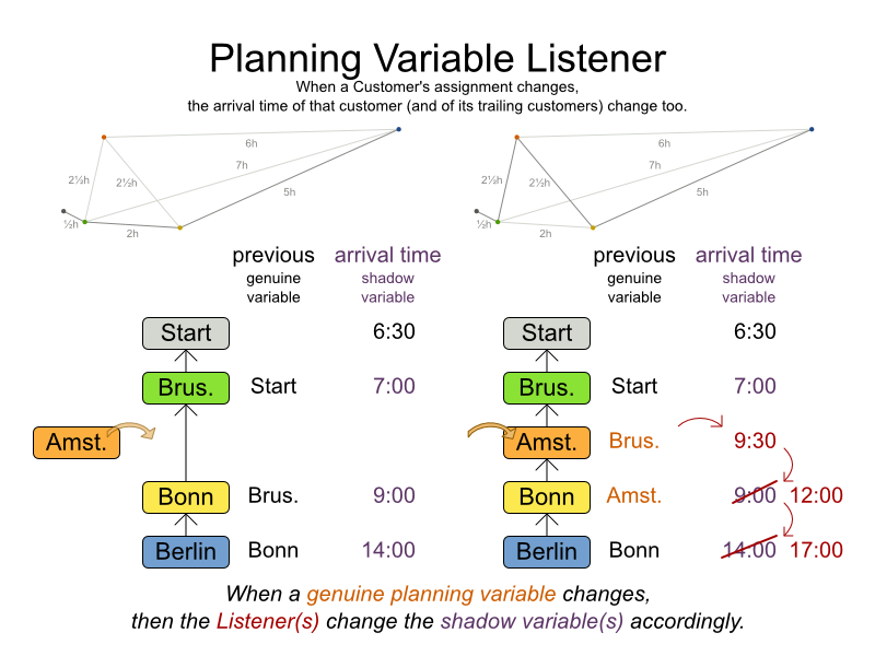
When the customers for a vehicle change, the arrival time for each customer is automatically adjusted. For more information, see the vehicle routing domain model.
From a score calculation perspective, a shadow variable is like any other planning variable. From an optimization perspective, Planner effectively only optimizes the genuine variables (and mostly ignores the shadow variables): it just assures that when a genuine variable changes, any dependent shadow variables are changed accordingly.
There are several build-in shadow variables:
2 variables are bi-directional if their instances always point to each other (unless one side points to
null and the other side doesn't exist). So if A references B, then B references A.
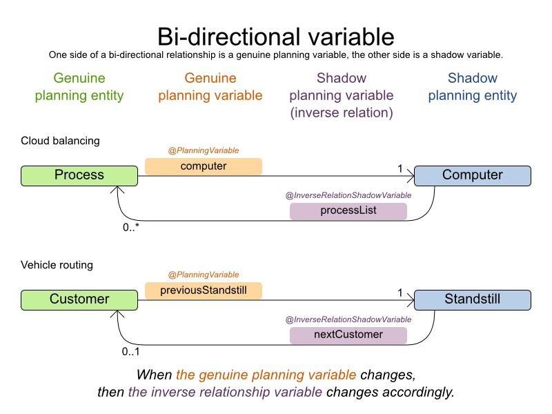
For a non-chained planning variable, the bi-directional relationship must be a many to one relationship. To map a bi-directional relationship between 2 planning variables, annotate the master side (which is the genuine side) as a normal planning variable:
@PlanningEntity
public class CloudProcess {
@PlanningVariable(...)
public CloudComputer getComputer() {
return computer;
}
public void setComputer(CloudComputer computer) {...}
}And then annotate the other side (which is the shadow side) with a
@InverseRelationShadowVariable annotation on a Collection (usually a
Set or List) property:
@PlanningEntity
public class CloudComputer {
@InverseRelationShadowVariable(sourceVariableName = "computer")
public List<CloudProcess> getProcessList() {
return processList;
}
}The sourceVariableName property is the name of the genuine planning variable on the
return type of the getter (so the name of the genuine planning variable on the other
side).
Note
The shadow property, which is a Collection, can never be null. If
no genuine variable is referencing that shadow entity, then it's an empty Collection.
Furthermore it must be a mutable Collection because once the Solver starts initializing or
changing genuine planning variables, it will add and remove to the Collections of those
shadow variables accordingly.
For a chained planning variable, the bi-directional relationship must be a one to one relationship. In that case, the genuine side looks like this:
@PlanningEntity
public class Customer ... {
@PlanningVariable(graphType = PlanningVariableGraphType.CHAINED, ...)
public Standstill getPreviousStandstill() {
return previousStandstill;
}
public void setPreviousStandstill(Standstill previousStandstill) {...}
}And the shadow side looks like this:
@PlanningEntity
public class Standstill {
@InverseRelationShadowVariable(sourceVariableName = "previousStandstill")
public Customer getNextCustomer() {
return nextCustomer;
}
public void setNextCustomer(Customer nextCustomer) {...}
}Warning
The input planning problem of a Solver must not violate bi-directional relationships.
If A points to B, then B must point to A. Planner will not violate that principle during planning, but the
input must not violate it.
An anchor shadow variable is the anchor of a chained variable.
Annotate the anchor property as a @AnchorShadowVariable annotation:
@PlanningEntity
public class Customer {
@AnchorShadowVariable(sourceVariableName = "previousStandstill")
public Vehicle getVehicle() {...}
public void setVehicle(Vehicle vehicle) {...}
}The sourceVariableName property is the name of the chained variable on the same entity
class.
To update a shadow variable, Planner uses a VariableListener. To define a custom shadow
variable, write a custom VariableListener: implement the interface and annotate it on the
shadow variable that needs to change.
@PlanningVariable(...)
public Standstill getPreviousStandstill() {
return previousStandstill;
}
@CustomShadowVariable(variableListenerClass = VehicleUpdatingVariableListener.class,
sources = {@CustomShadowVariable.Source(variableName = "previousStandstill")})
public Vehicle getVehicle() {
return vehicle;
}The variableName is the variable that triggers changes in the shadow
variable(s).
Note
If the class of the trigger variable is different than the shadow variable, also specify the
entityClass on @CustomShadowVariable.Source. In that case, make sure
that that entityClass is also properly configured as a planning entity class in the solver
config, or the VariableListener will simply never trigger.
Any class that has at least 1 shadow variable, is a planning entity class, even it has no genuine planning variables.
For example, the VehicleUpdatingVariableListener assures that every
Customer in a chain has the same Vehicle, namely the chain's
anchor.
public class VehicleUpdatingVariableListener implements VariableListener<Customer> {
public void afterEntityAdded(ScoreDirector scoreDirector, Customer customer) {
updateVehicle(scoreDirector, customer);
}
public void afterVariableChanged(ScoreDirector scoreDirector, Customer customer) {
updateVehicle(scoreDirector, customer);
}
...
protected void updateVehicle(ScoreDirector scoreDirector, Customer sourceCustomer) {
Standstill previousStandstill = sourceCustomer.getPreviousStandstill();
Vehicle vehicle = previousStandstill == null ? null : previousStandstill.getVehicle();
Customer shadowCustomer = sourceCustomer;
while (shadowCustomer != null && shadowCustomer.getVehicle() != vehicle) {
scoreDirector.beforeVariableChanged(shadowCustomer, "vehicle");
shadowCustomer.setVehicle(vehicle);
scoreDirector.afterVariableChanged(shadowCustomer, "vehicle");
shadowCustomer = shadowCustomer.getNextCustomer();
}
}
}Warning
A VariableListener can only change shadow variables. It must never change a genuine
planning variable or a problem fact.
Warning
Any change of a shadow variable must be told to the ScoreDirector.
A dataset for a planning problem needs to be wrapped in a class for the Solver to
solve. You must implement this class. For example in n queens, this in the NQueens class
which contains a Column list, a Row list and a Queen
list.
A planning problem is actually a unsolved planning solution or - stated differently - an uninitialized
Solution. Therefore, that wrapping class must implement the Solution
interface. For example in n queens, that NQueens class implements
Solution, yet every Queen in a fresh NQueens class is
not yet assigned to a Row (their row property is null).
So it's not a feasible solution. It's not even a possible solution. It's an uninitialized solution.
You need to present the problem as a Solution instance to the
Solver. So your class needs to implement the Solution interface:
public interface Solution<S extends Score> {
S getScore();
void setScore(S score);
Collection<? extends Object> getProblemFacts();
}For example, an NQueens instance holds a list of all columns, all rows and all
Queen instances:
@PlanningSolution
public class NQueens implements Solution<SimpleScore> {
private int n;
// Problem facts
private List<Column> columnList;
private List<Row> rowList;
// Planning entities
private List<Queen> queenList;
// ...
}A Solution requires a score property. The score property is null if
the Solution is uninitialized or if the score has not yet been (re)calculated. The
score property is usually typed to the specific Score implementation you
use. For example, NQueens uses a SimpleScore:
@PlanningSolution
public class NQueens implements Solution<SimpleScore> {
private SimpleScore score;
public SimpleScore getScore() {
return score;
}
public void setScore(SimpleScore score) {
this.score = score;
}
// ...
}Most use cases use a HardSoftScore instead:
@PlanningSolution
public class CourseSchedule implements Solution<HardSoftScore> {
private HardSoftScore score;
public HardSoftScore getScore() {
return score;
}
public void setScore(HardSoftScore score) {
this.score = score;
}
// ...
}See the Score calculation section for more information on the Score
implementations.
The method is only used if Drools is used for score calculation. Other score directors do not use it.
All objects returned by the getProblemFacts() method will be asserted into the Drools
working memory, so the score rules can access them. For example, NQueens just returns all
Column and Row instances.
public Collection<? extends Object> getProblemFacts() {
List<Object> facts = new ArrayList<Object>();
facts.addAll(columnList);
facts.addAll(rowList);
// Do not add the planning entity's (queenList) because that will be done automatically
return facts;
}All planning entities are automatically inserted into the Drools working memory. Do
not add them in the method getProblemFacts().
Note
A common mistake is to use facts.add(...) instead of
fact.addAll(...) for a Collection, which leads to score rules failing to
match because the elements of that Collection aren't in the Drools working memory.
The getProblemFacts() method is not called much: at most only once per solver phase per
solver thread.
A cached problem fact is a problem fact that doesn't exist in the real domain model, but is calculated
before the Solver really starts solving. The getProblemFacts() method
has the chance to enrich the domain model with such cached problem facts, which can lead to simpler and faster
score constraints.
For example in examination, a cached problem fact TopicConflict is created for every
2 Topic's which share at least 1 Student.
public Collection<? extends Object> getProblemFacts() {
List<Object> facts = new ArrayList<Object>();
// ...
facts.addAll(calculateTopicConflictList());
// ...
return facts;
}
private List<TopicConflict> calculateTopicConflictList() {
List<TopicConflict> topicConflictList = new ArrayList<TopicConflict>();
for (Topic leftTopic : topicList) {
for (Topic rightTopic : topicList) {
if (leftTopic.getId() < rightTopic.getId()) {
int studentSize = 0;
for (Student student : leftTopic.getStudentList()) {
if (rightTopic.getStudentList().contains(student)) {
studentSize++;
}
}
if (studentSize > 0) {
topicConflictList.add(new TopicConflict(leftTopic, rightTopic, studentSize));
}
}
}
}
return topicConflictList;
}Any score constraint that needs to check if no 2 exams have a topic which share a student are being
scheduled close together (depending on the constraint: at the same time, in a row or in the same day), can
simply use the TopicConflict instance as a problem fact, instead of having to combine every
2 Student instances.
Planner needs to extract the entity instances from the Solution instance. It gets those
collection(s) by calling every getter (or field) that is annotated with
@PlanningEntityCollectionProperty:
@PlanningSolution
public class NQueens implements Solution<SimpleScore> {
...
private List<Queen> queenList;
@PlanningEntityCollectionProperty
public List<Queen> getQueenList() {
return queenList;
}
}There can be multiple @PlanningEntityCollectionProperty annotated members. Those can
even return a Collection with the same entity class type.
In rare cases, a planning entity might be a singleton: use @PlanningEntityProperty on
its getter (or field) instead.
Most (if not all) optimization algorithms clone the solution each time they encounter a new best solution (so they can recall it later) or to work with multiple solutions in parallel.
Note
There are many ways to clone, such as a shallow clone, deep clone, ... This context focuses on a planning clone.
A planning clone of a Solution must fulfill these requirements:
The clone must represent the same planning problem. Usually it reuses the same instances of the problem facts and problem fact collections as the original.
The clone must use different, cloned instances of the entities and entity collections. Changes to an original
Solution's entity's variables must not effect its clone.
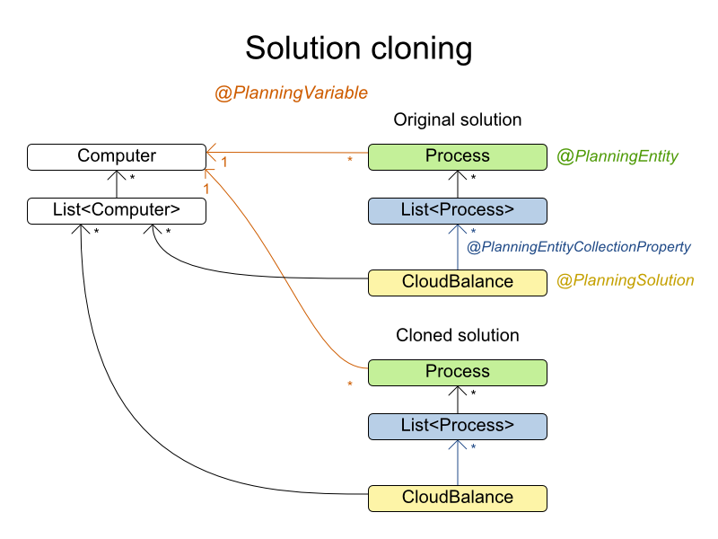
Implementing a planning clone method is hard, therefore you don't need to implement it.
This SolutionCloner is used by default. It works well for most use cases.
Warning
When the FieldAccessingSolutionCloner clones your entity collection, it might not
recognize the implementation and replace it with ArrayList,
LinkedHashSet or TreeSet (whichever is more applicable). It recognizes
most of the common JDK Collection implementations.
The FieldAccessingSolutionCloner does not clone problem facts by default. If any of
your problem facts needs to be deep cloned for a planning clone, for example if the problem fact references a
planning entity or the planning solution, mark it with a @DeepPlanningClone
annotation:
@DeepPlanningClone
public class SeatDesignationDependency {
private SeatDesignation leftSeatDesignation; // planning entity
private SeatDesignation rightSeatDesignation; // planning entity
...
}In the example above, because SeatDesignation is a planning entity (which is deep
planning cloned automatically), SeatDesignationDependency must be deep planning cloned
too.
Alternatively, the @DeepPlanningClone annotation can also be used on a getter
method.
If your Solution implements PlanningCloneable, Planner will
automatically choose to clone it by calling the planningClone() method.
public interface PlanningCloneable<T> {
T planningClone();
}For example: If NQueens implements PlanningCloneable, it would
only deep clone all Queen instances. When the original solution is changed during planning,
by changing a Queen, the clone stays the same.
public class NQueens implements Solution<...>, PlanningCloneable<NQueens> {
...
/**
* Clone will only deep copy the {@link #queenList}.
*/
public NQueens planningClone() {
NQueens clone = new NQueens();
clone.id = id;
clone.n = n;
clone.columnList = columnList;
clone.rowList = rowList;
List<Queen> clonedQueenList = new ArrayList<Queen>(queenList.size());
for (Queen queen : queenList) {
clonedQueenList.add(queen.planningClone());
}
clone.queenList = clonedQueenList;
clone.score = score;
return clone;
}
}The planningClone() method should only deep clone the planning
entities. Notice that the problem facts, such as Column and
Row are normally not cloned: even their List
instances are not cloned. If you were to clone the problem facts too, then you'd have to
make sure that the new planning entity clones also refer to the new problem facts clones used by the solution.
For example, if you would clone all Row instances, then each Queen clone
and the NQueens clone itself should refer to those new Row
clones.
Warning
Cloning an entity with a chained variable is devious: a variable of an entity A might point to another entity B. If A is cloned, then it's variable must point to the clone of B, not the original B.
Create a Solution instance to represent your planning problem's dataset, so it can be
set on the Solver as the planning problem to solve. For example in n queens, an
NQueens instance is created with the required Column and
Row instances and every Queen set to a different column
and every row set to null.
private NQueens createNQueens(int n) {
NQueens nQueens = new NQueens();
nQueens.setId(0L);
nQueens.setN(n);
nQueens.setColumnList(createColumnList(nQueens));
nQueens.setRowList(createRowList(nQueens));
nQueens.setQueenList(createQueenList(nQueens));
return nQueens;
}
private List<Queen> createQueenList(NQueens nQueens) {
int n = nQueens.getN();
List<Queen> queenList = new ArrayList<Queen>(n);
long id = 0L;
for (Column column : nQueens.getColumnList()) {
Queen queen = new Queen();
queen.setId(id);
id++;
queen.setColumn(column);
// Notice that we leave the PlanningVariable properties on null
queenList.add(queen);
}
return queenList;
}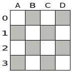
Usually, most of this data comes from your data layer, and your Solution implementation
just aggregates that data and creates the uninitialized planning entity instances to plan:
private void createLectureList(CourseSchedule schedule) {
List<Course> courseList = schedule.getCourseList();
List<Lecture> lectureList = new ArrayList<Lecture>(courseList.size());
long id = 0L;
for (Course course : courseList) {
for (int i = 0; i < course.getLectureSize(); i++) {
Lecture lecture = new Lecture();
lecture.setId(id);
id++;
lecture.setCourse(course);
lecture.setLectureIndexInCourse(i);
// Notice that we leave the PlanningVariable properties (period and room) on null
lectureList.add(lecture);
}
}
schedule.setLectureList(lectureList);
}A Solver implementation will solve your planning problem.
public interface Solver {
void solve(Solution planningProblem);
Solution getBestSolution();
// ...
}A Solver can only solve 1 planning problem instance at a time. A
Solver should only be accessed from a single thread, except for the methods that are
specifically javadocced as being thread-safe. It's built with a SolverFactory, do not implement
or build it yourself.
Solving a problem is quite easy once you have:
A
Solverbuilt from a solver configurationA
Solutionthat represents the planning problem instance
Just set the planning problem, solve it and extract the best solution:
solver.solve(planningProblem);
Solution bestSolution = solver.getBestSolution();For example in n queens, the getBestSolution() method will return an
NQueens instance with every Queen assigned to a
Row.

The solve(Solution) method can take a long time (depending on the problem size and the
solver configuration). The Solver will remember (actually clone) the best solution it
encounters during its solving. Depending on a number factors (including problem size, how much time the
Solver has, the solver configuration, ...), that best solution will be a feasible or even an
optimal solution.
Note
The Solution instance given to the method solve(Solution) will be
changed by the Solver, but do not mistake it for the best solution.
The Solution instance returned by the getBestSolution() method will
most likely be a clone of the instance given to the method solve(Solution), which means it's
a different instance.
Note
The Solution instance given to the solve(Solution) method does not
need to be uninitialized. It can be partially or fully initialized, which is likely to be the case in repeated planning.
The environment mode allows you to detect common bugs in your implementation. It does not affect the logging level.
You can set the environment mode in the solver configuration XML file:
<solver>
<environmentMode>FAST_ASSERT</environmentMode>
...
</solver>A solver has a single Random instance. Some solver configurations use the
Random instance a lot more than others. For example Simulated Annealing depends highly on
random numbers, while Tabu Search only depends on it to deal with score ties. The environment mode influences the
seed of that Random instance.
These are the environment modes:
The FULL_ASSERT mode turns on all assertions (such as assert that the incremental score calculation is uncorrupted for each move) to fail-fast on a bug in a Move implementation, a score rule, the rule engine itself, ...
This mode is reproducible (see the reproducible mode). It is also intrusive because it calls the method
calculateScore() more frequently than a non assert mode.
The FULL_ASSERT mode is horribly slow (because it doesn't rely on incremental score calculation).
The NON_INTRUSIVE_FULL_ASSERT turns on several assertions to fail-fast on a bug in a Move implementation, a score rule, the rule engine itself, ...
This mode is reproducible (see the reproducible mode). It is non-intrusive because it does not call the
method calculateScore() more frequently than a non assert mode.
The NON_INTRUSIVE_FULL_ASSERT mode is horribly slow (because it doesn't rely on incremental score calculation).
The FAST_ASSERT mode turns on most assertions (such as assert that an undoMove's score is the same as before the Move) to fail-fast on a bug in a Move implementation, a score rule, the rule engine itself, ...
This mode is reproducible (see the reproducible mode). It is also intrusive because it calls the method
calculateScore() more frequently than a non assert mode.
The FAST_ASSERT mode is slow.
It's recommended to write a test case which does a short run of your planning problem with the FAST_ASSERT mode on.
The reproducible mode is the default mode because it is recommended during development. In this mode, 2 runs in the same Planner version will execute the same code in the same order. Those 2 runs will have the same result at every step, except if the note below applies. This enables you to reproduce bugs consistently. It also allows you to benchmark certain refactorings (such as a score constraint performance optimization) fairly across runs.
Note
Despite the reproducible mode, your application might still not be fully reproducible because of:
Use of
HashSet(or anotherCollectionwhich has an inconsistent order between JVM runs) for collections of planning entities or planning values (but not normal problem facts), especially in theSolutionimplementation. Replace it withLinkedHashSet.Combining a time gradient dependent algorithms (most notably Simulated Annealing) together with time spent termination. A sufficiently large difference in allocated CPU time will influence the time gradient values. Replace Simulated Annealing with Late Acceptance. Or instead, replace time spent termination with step count termination.
The reproducible mode is slightly slower than the production mode. If your production environment requires reproducibility, use this mode in production too.
In practice, this mode uses the default, fixed random seed if no seed is specified, and it also disables certain concurrency optimizations (such as work stealing).
The production mode is the fastest, but it is not reproducible. It is recommended for a production environment, unless reproducibility is required.
In practice, this mode uses no fixed random seed if no seed is specified.
The best way to illuminate the black box that is a Solver, is to play with the logging
level:
error: Log errors, except those that are thrown to the calling code as a
RuntimeException.Note
If an error happens, Planner normally fails fast: it throws a subclass of
RuntimeExceptionwith a detailed message to the calling code. It does not log it as an error itself to avoid duplicate log messages. Except if the calling code explicitly catches and eats thatRuntimeException, aThread's defaultExceptionHandlerwill log it as an error anyway. Meanwhile, the code is disrupted from doing further harm or obfuscating the error.warn: Log suspicious circumstances.
info: Log every phase and the solver itself. See scope overview.
debug: Log every step of every phase. See scope overview.
trace: Log every move of every step of every phase. See scope overview.
Note
Turning on
tracelogging, will slow down performance considerably: it's often 4 times slower. However, it's invaluable during development to discover a bottleneck.Even debug logging can slow down performance considerably for fast stepping algorithms (such as Late Acceptance and Simulated Annealing), but not for slow stepping algorithms (such as Tabu Search).
For example, set it to debug logging, to see when the phases end and how fast steps are
taken:
INFO Solving started: time spent (3), best score (uninitialized/0), random (JDK with seed 0).
DEBUG CH step (0), time spent (5), score (0), selected move count (1), picked move (Queen-2 {null -> Row-0}).
DEBUG CH step (1), time spent (7), score (0), selected move count (3), picked move (Queen-1 {null -> Row-2}).
DEBUG CH step (2), time spent (10), score (0), selected move count (4), picked move (Queen-3 {null -> Row-3}).
DEBUG CH step (3), time spent (12), score (-1), selected move count (4), picked move (Queen-0 {null -> Row-1}).
INFO Construction Heuristic phase (0) ended: step total (4), time spent (12), best score (-1).
DEBUG LS step (0), time spent (19), score (-1), best score (-1), accepted/selected move count (12/12), picked move (Queen-1 {Row-2 -> Row-3}).
DEBUG LS step (1), time spent (24), score (0), new best score (0), accepted/selected move count (9/12), picked move (Queen-3 {Row-3 -> Row-2}).
INFO Local Search phase (1) ended: step total (2), time spent (24), best score (0).
INFO Solving ended: time spent (24), best score (0), average calculate count per second (1625).All time spent values are in milliseconds.
Everything is logged to SLF4J, which is a simple logging facade which delegates every log message to Logback, Apache Commons Logging, Log4j or java.util.logging. Add a dependency to the logging adaptor for your logging framework of choice.
If you're not using any logging framework yet, use Logback by adding this Maven dependency (there is no need to add an extra bridge dependency):
<dependency>
<groupId>ch.qos.logback</groupId>
<artifactId>logback-classic</artifactId>
<version>1.x</version>
</dependency>Configure the logging level on the org.optaplanner package in your
logback.xml file:
<configuration>
<logger name="org.optaplanner" level="debug"/>
...
<configuration>If instead, you're still using Log4J 1.x (and you don't want to switch to its faster successor, Logback), add the bridge dependency:
<dependency>
<groupId>org.slf4j</groupId>
<artifactId>slf4j-log4j12</artifactId>
<version>1.x</version>
</dependency>And configure the logging level on the package org.optaplanner in your
log4j.xml file:
<log4j:configuration xmlns:log4j="http://jakarta.apache.org/log4j/">
<category name="org.optaplanner">
<priority value="debug" />
</category>
...
</log4j:configuration>Note
In a multitenant application, multiple Solver instances might be running at the same
time. To separate their logging into distinct files, surround the solve() call with an MDC:
MDC.put("tenant.name",tenantName);
solver.solve(planningProblem);
Solution bestSolution = solver.getBestSolution();
MDC.remove("tenant.name");Then configure your logger to use different files for each ${tenant.name}. For example
in Logback, use a SiftingAppender in logback.xml:
<appender name="fileAppender" class="ch.qos.logback.classic.sift.SiftingAppender">
<discriminator>
<key>tenant.name</key>
<defaultValue>unknown</defaultValue>
</discriminator>
<sift>
<appender name="fileAppender.${tenant.name}" class="...FileAppender">
<file>local/log/optaplanner-${tenant.name}.log</file>
...
</appender>
</sift>
</appender>Many heuristics and metaheuristics depend on a pseudorandom number generator for move selection, to resolve
score ties, probability based move acceptance, ... During solving, the same Random instance is
reused to improve reproducibility, performance and uniform distribution of random values.
To change the random seed of that Random instance, specify a
randomSeed:
<solver>
<randomSeed>0</randomSeed>
...
</solver>To change the pseudorandom number generator implementation, specify a randomType:
<solver>
<randomType>MERSENNE_TWISTER</randomType>
...
</solver>The following types are supported:
JDK(default): Standard implementation (java.util.Random).MERSENNE_TWISTER: Implementation by Commons Math.WELL512A,WELL1024A,WELL19937A,WELL19937C,WELL44497AandWELL44497B: Implementation by Commons Math.
For most use cases, the randomType has no significant impact on the average quality of the best solution on multiple datasets. If you want to confirm this on your use case, use the benchmarker.
- 5.1. Score Terminology
- 5.2. Choose a Score Definition
- 5.3. Calculate the
Score - 5.4. Score Calculation Performance Tricks
- 5.4.1. Overview
- 5.4.2. Average Calculation Count Per Second
- 5.4.3. Incremental Score Calculation (with Delta's)
- 5.4.4. Avoid Calling Remote Services During Score Calculation
- 5.4.5. Pointless Constraints
- 5.4.6. Built-in Hard Constraint
- 5.4.7. Other Score Calculation Performance Tricks
- 5.4.8. Score Trap
- 5.4.9. stepLimit Benchmark
- 5.4.10. Fairness Score Constraints
- 5.5. Explaining the Score: Using Score Calculation Outside the
Solver
Every initialized Solution has a score. That score is an objective way to compare 2
solutions: the solution with the higher score is better. The Solver aims to find the
Solution with the highest Score of all possible solutions. The
best solution is the Solution with the highest Score
that Solver has encountered during solving, which might be the optimal
solution.
Planner cannot automatically know which Solution is best for your business, so you need
to tell it how to calculate the score of a given Solution according to your business needs. If
you forget or unable to implement an important constraint, the solution is probably useless:
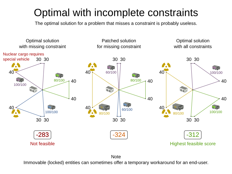
Luckily, Planner is very flexible to define constraints, thanks to these score techniques, which can be used and combined as much as needed:
Score signum (positive or negative): maximize or minimize a constraint type.
Score weight: put a cost/profit on a constraint type.
Score level: prioritize a group of constraint types
Pareto scoring
All score techniques are based on constraints. Such a constraint can be a simple pattern (such as Maximize the apple harvest in the solution) or a more complex pattern. A positive constraint is a constraint you're trying to maximize. A negative constraint is a constraint you're trying to minimize.
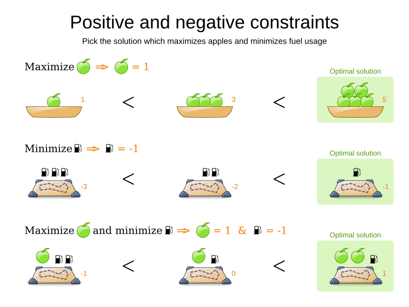
Notice in the image above, that the optimal solution always has the highest score, regardless if the constraints are positive or negative.
Most planning problems have only negative constraints and therefore have a negative score. In that case, the score is usually the sum of the weight of the negative constraints being broken, with a perfect score of 0. This explains why the score of a solution of 4 queens is the negative (and not the positive!) of the number of queen pairs which can attack each other.
Negative and positive constraints can be combined, even in the same score level.
Note
Don't presume your business knows all its score constraints in advance. Expect score constraints to be added or changed after the first releases.
When a constraint activates (because the negative constraint is broken or the positive constraint is fulfilled) on a certain planning entity set, it is called a constraint match.
Not all score constraints are equally important. If breaking one constraint is equally bad as breaking another constraint x times, then those 2 constraints have a different weight (but they are in the same score level). For example in vehicle routing, you can make1 "unhappy driver" constraint match count as much as 2 "fuel tank usage" constraint matches:
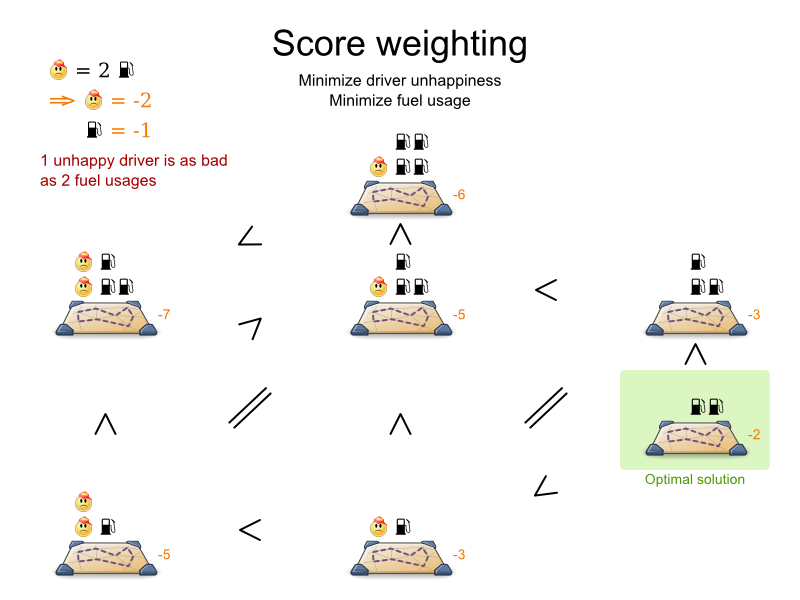
Score weighting is often used in use cases where you can put a price tag on everything. In that case, the positive constraints maximize revenue and the negative constraints minimize expenses: together they maximize profit. Alternatively, score weighting is also often used to create social fairness. For example: a nurse that requests a free day pays a higher weight on New Year's eve than on a normal day.
Put a good weight on a constraint can be a difficult analytical decision, because it's about making choices and tradeoffs with other constraints. However, a non-accurate weight is less damaging than not good algorithms:
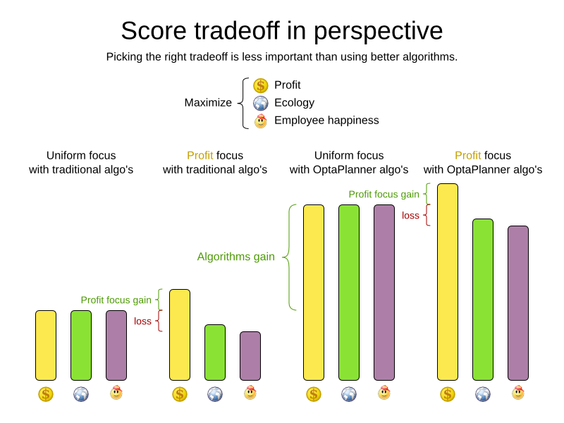
Furthermore, it is often useful to allow the planning end-user to recalibrate penalty weights in his/her user interface, as demonstrated in the exam timetabling example.
The weight of a constraint match can be dynamically based on the planning entities involved. For example in
cloud balance: the weight of the soft constraint match for an active Computer is the
cost of that Computer.
Sometimes a score constraint outranks another score constraint, no matter how many times the other is broken. In that case, those score constraints are in different levels. For example: a nurse cannot do 2 shifts at the same time (due to the constraints of physical reality), this outranks all nurse happiness constraints.
Most use cases have only 2 score levels: hard and soft. When comparing 2 scores, they are compared lexicographically: the first score level gets compared first. If those differ, the others score levels are ignored. For example: a score that breaks 0 hard constraints and 1000000 soft constraints is better than a score that breaks 1 hard constraint and 0 soft constraints.
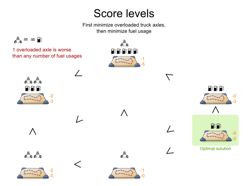
Score levels often employ score weighting per level. In such case, the hard constraint level usually makes the solution feasible and the soft constraint level maximizes profit by weighting the constraints on price.
Don't use a big constraint weight when your business actually wants different score levels. That hack, known as score folding, is broken:
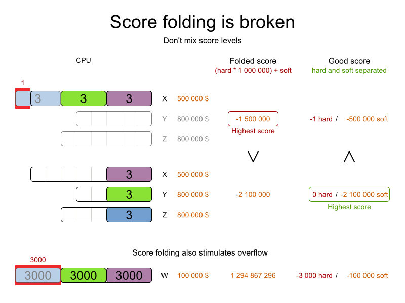
Note
Your business will probably tell you that your hard constraints all have the same weight, because they
cannot be broken (so their weight does not matter). This is not true and it could create a score trap. For example in cloud balance: if a Computer has 7 CPU
too little for its Processes, then it must be weighted 7 times as much as if it had only 1
CPU too little. This way, there is an incentive to move a Process with 6 CPU or less away
from that Computer.
Three or more score levels are also supported. For example: a company might decide that profit outranks employee satisfaction (or visa versa), while both are outranked by the constraints of physical reality.
Note
To model fairness or load balancing, there is no need to use lots of score levels (even though Planner can handle many score levels).
Far less common is the use case of pareto optimization, which is also known under the more confusing term multi-objective optimization. In pareto scoring, score constraints are in the same score level, yet they are not weighted against each other. When 2 scores are compared, each of the score constraints are compared individually and the score with the most dominating score constraints wins. Pareto scoring can even be combined with score levels and score constraint weighting.
Consider this example with positive constraints, where we want to get the most apples and oranges. Since it's impossible to compare apples and oranges, we can't weight them against each other. Yet, despite that we can't compare them, we can state that 2 apples are better then 1 apple. Similarly, we can state that 2 apples and 1 orange are better than just 1 orange. So despite our inability to compare some Scores conclusively (at which point we declare them equal), we can find a set of optimal scores. Those are called pareto optimal.
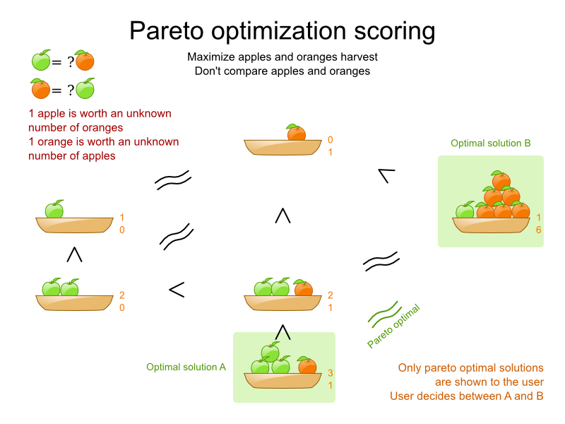
Scores are considered equal far more often. It's left up to a human to choose the better out of a set of best solutions (with equal scores) found by Planner. In the example above, the user must choose between solution A (3 apples and 1 orange) and solution B (1 apple and 6 oranges). It's guaranteed that Planner has not found another solution which has more apples or more oranges or even a better combination of both (such as 2 apples and 3 oranges).
To implement pareto scoring in Planner, implement a custom
ScoreDefinition and Score (and replace the
BestSolutionRecaller). Future versions will provide out-of-the-box support.
Note
A pareto Score's compareTo method is not transitive because it does
a pareto comparison. For example: having 2 apples is greater than 1 apple. 1 apple is equal to 1 orange. Yet, 2
apples are not greater than 1 orange (but actually equal). Pareto comparison violates the contract of the
interface java.lang.Comparable's compareTo method, but Planner's systems
are pareto comparison safe, unless explicitly stated otherwise in this
documentation.
All the score techniques mentioned above, can be combined seamlessly:
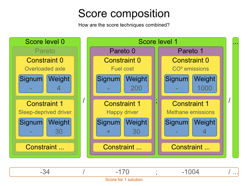
A score is represented by the Score interface, which naturally extends
Comparable:
public interface Score<...> extends Comparable<...> {
...
}The Score implementation to use depends on your use case. Your score might not
efficiently fit in a single long value. Planner has several built-in Score
implementations, but you can implement a custom Score too. Most use cases tend to use the
built-in HardSoftScore.
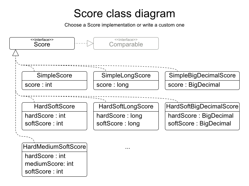
The Score implementation (for example HardSoftScore) must be the same
throughout a Solver runtime. The Score implementation is configured in the
solver configuration as a ScoreDefinition:
<scoreDirectorFactory>
<scoreDefinitionType>HARD_SOFT</scoreDefinitionType>
...
</scoreDirectorFactory>Avoid the use of float and double for score calculation. Use
BigDecimal instead.
Floating point numbers (float and double) cannot represent a decimal
number correctly. For example: a double cannot hold the value 0.05
correctly. Instead, it holds the nearest representable value. Arithmetic (including addition and subtraction) with
floating point numbers, especially for planning problems, leads to incorrect decisions:
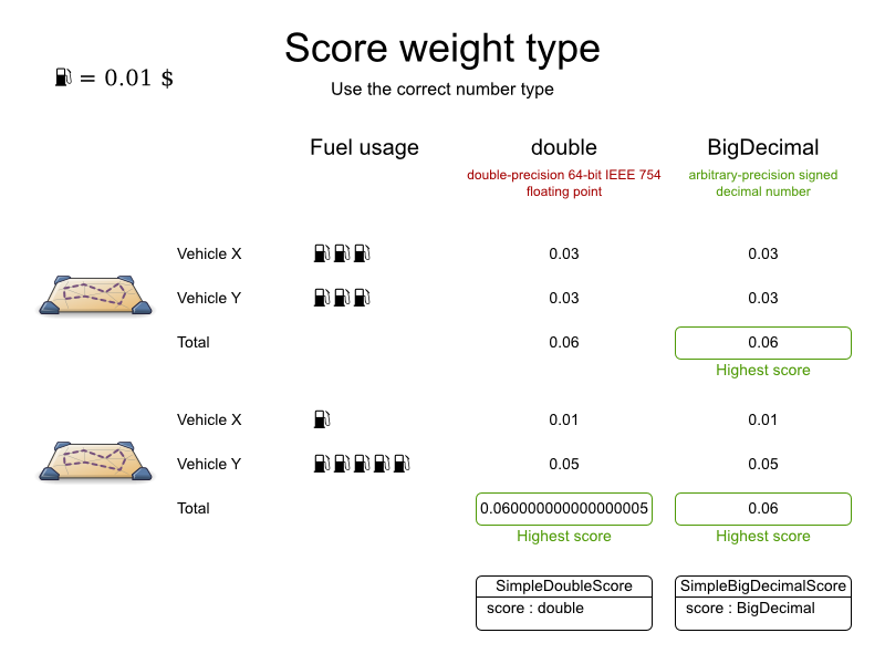
Additionally, floating point number addition is not associative:
System.out.println( ((0.01 + 0.02) + 0.03) == (0.01 + (0.02 + 0.03)) ); // returns falseThis leads to score corruption.
Decimal numbers (BigDecimal) have none of these problems.
Note
BigDecimal arithmetic is considerably slower than int, long or
double arithmetic. In experiments we've seen the average calculation count get divided by
5.
Therefore, in some cases, it can be worthwhile to multiply all numbers for a single
score weight by a plural of ten (for example 1000), so the score weight fits in an
int or long.
Each Score implementation also has a ScoreDefinition implementation. For
example: SimpleScore is defined by SimpleScoreDefinition.
A SimpleScore has a single int value, for example
-123. It has a single score level.
<scoreDirectorFactory>
<scoreDefinitionType>SIMPLE</scoreDefinitionType>
...
</scoreDirectorFactory>Variants of this scoreDefinitionType:
SIMPLE_LONG: UsesSimpleLongScorewhich has alongvalue instead of anintvalue.SIMPLE_DOUBLE: UsesSimpleDoubleScorewhich has adoublevalue instead of anintvalue. Not recommended to use.SIMPLE_BIG_DECIMAL: UsesSimpleBigDecimalScorewhich has aBigDecimalvalue instead of anintvalue.
A HardSoftScore has a hard int value and a soft int
value, for example -123hard/-456soft. It has 2 score levels (hard and soft).
<scoreDirectorFactory>
<scoreDefinitionType>HARD_SOFT</scoreDefinitionType>
...
</scoreDirectorFactory>Variants of this scoreDefinitionType:
HARD_SOFT_LONG: UsesHardSoftLongScorewhich haslongvalues instead ofintvalues.HARD_SOFT_DOUBLE: UsesHardSoftDoubleScorewhich hasdoublevalues instead ofintvalues. Not recommended to use.HARD_SOFT_BIG_DECIMAL: UsesHardSoftBigDecimalScorewhich hasBigDecimalvalues instead ofintvalues.
A HardMediumSoftScore which has a hard int value, a medium
int value and a soft int value, for example
-123hard/-456medium/-789soft. It has 3 score levels (hard, medium and soft).
<scoreDirectorFactory>
<scoreDefinitionType>HARD_MEDIUM_SOFT</scoreDefinitionType>
...
</scoreDirectorFactory>Variants of this scoreDefinitionType:
HARD_MEDIUM_SOFT_LONG: UsesHardMediumSoftLongScorewhich haslongvalues instead ofintvalues.
A BendableScore has a configurable number of score levels. It has an array of hard
int values and an array of soft int value, for example with 2 hard levels
and 3 soft levels, the score can be -123/-456/-789/-012/-345.
<scoreDirectorFactory>
<scoreDefinitionType>BENDABLE</scoreDefinitionType>
<bendableHardLevelsSize>2</bendableHardLevelsSize>
<bendableSoftLevelsSize>3</bendableSoftLevelsSize>
...
</scoreDirectorFactory>The number of hard and soft score levels needs to be set at configuration time: it's not flexible to change during solving.
Variants of this scoreDefinitionType:
BENDABLE_Long: UsesBendableLongScorewhich haslongvalues instead ofintvalues.BENDABLE_BIG_DECIMAL: UsesBendableBigDecimalScorewhich hasBigDecimalvalues instead ofintvalues.
The ScoreDefinition interface defines the score representation.
To implement a custom Score, you'll also need to implement a custom
ScoreDefinition. Extend AbstractScoreDefinition (preferably by copy pasting
HardSoftScoreDefinition) and start from there.
Then hook your custom ScoreDefinition in your
SolverConfig.xml:
<scoreDirectorFactory>
<scoreDefinitionClass>...MyScoreDefinition</scoreDefinitionClass>
...
</scoreDirectorFactory>There are several ways to calculate the Score of a Solution:
Easy Java score calculation: implement a single Java method
Incremental Java score calculation: implement multiple Java methods
Drools score calculation (recommended): implement score rules
Every score calculation type can use any Score definition. For example, easy Java score calculation can
output a HardSoftScore.
All score calculation types are Object Oriented and can reuse existing Java code.
Important
The score calculation should be read-only: it should not change the planning entities or the problem facts in any way. For example, it must not call a setter method on a planning entity in a Drools score rule's RHS. This does not apply to logically inserted objects, which can be changed by the score rules that logically inserted them in the first place.
Planner will not recalculate the score of a Solution if it can predict it (unless an
environmentMode assertion is enabled). For example, after a winning step
is done, there is no need to calculate the score because that move was done and undone earlier. As a result,
there's no guarantee that such changes applied during score calculation are actually done.
An easy way to implement your score calculation in Java.
Advantages:
Plain old Java: no learning curve
Opportunity to delegate score calculation to an existing code base or legacy system
Disadvantages:
Slower and less scalable
Because there is no incremental score calculation
Just implement one method of the interface EasyScoreCalculator:
public interface EasyScoreCalculator<Sol extends Solution> {
Score calculateScore(Sol solution);
}For example in n queens:
public class NQueensEasyScoreCalculator implements EasyScoreCalculator<NQueens> {
public SimpleScore calculateScore(NQueens nQueens) {
int n = nQueens.getN();
List<Queen> queenList = nQueens.getQueenList();
int score = 0;
for (int i = 0; i < n; i++) {
for (int j = i + 1; j < n; j++) {
Queen leftQueen = queenList.get(i);
Queen rightQueen = queenList.get(j);
if (leftQueen.getRow() != null && rightQueen.getRow() != null) {
if (leftQueen.getRowIndex() == rightQueen.getRowIndex()) {
score--;
}
if (leftQueen.getAscendingDiagonalIndex() == rightQueen.getAscendingDiagonalIndex()) {
score--;
}
if (leftQueen.getDescendingDiagonalIndex() == rightQueen.getDescendingDiagonalIndex()) {
score--;
}
}
}
}
return SimpleScore.valueOf(score);
}
}Configure it in your solver configuration:
<scoreDirectorFactory>
<scoreDefinitionType>...</scoreDefinitionType>
<easyScoreCalculatorClass>org.optaplanner.examples.nqueens.solver.score.NQueensEasyScoreCalculator</easyScoreCalculatorClass>
</scoreDirectorFactory>Alternatively, build a EasyScoreCalculator instance at runtime and set it with the
programmatic API:
solverFactory.getSolverConfig().getScoreDirectorFactoryConfig.setEasyScoreCalculator(easyScoreCalculator);A way to implement your score calculation incrementally in Java.
Advantages:
Very fast and scalable
Currently the fastest if implemented correctly
Disadvantages:
Hard to write
A scalable implementation heavily uses maps, indexes, ... (things the Drools rule engine can do for you)
You have to learn, design, write and improve all these performance optimizations yourself
Hard to read
Regular score constraint changes can lead to a high maintenance cost
Implement all the methods of the interface IncrementalScoreCalculator and extend the
class AbstractIncrementalScoreCalculator:
public interface IncrementalScoreCalculator<Sol extends Solution> {
void resetWorkingSolution(Sol workingSolution);
void beforeEntityAdded(Object entity);
void afterEntityAdded(Object entity);
void beforeVariableChanged(Object entity, String variableName);
void afterVariableChanged(Object entity, String variableName);
void beforeEntityRemoved(Object entity);
void afterEntityRemoved(Object entity);
Score calculateScore();
}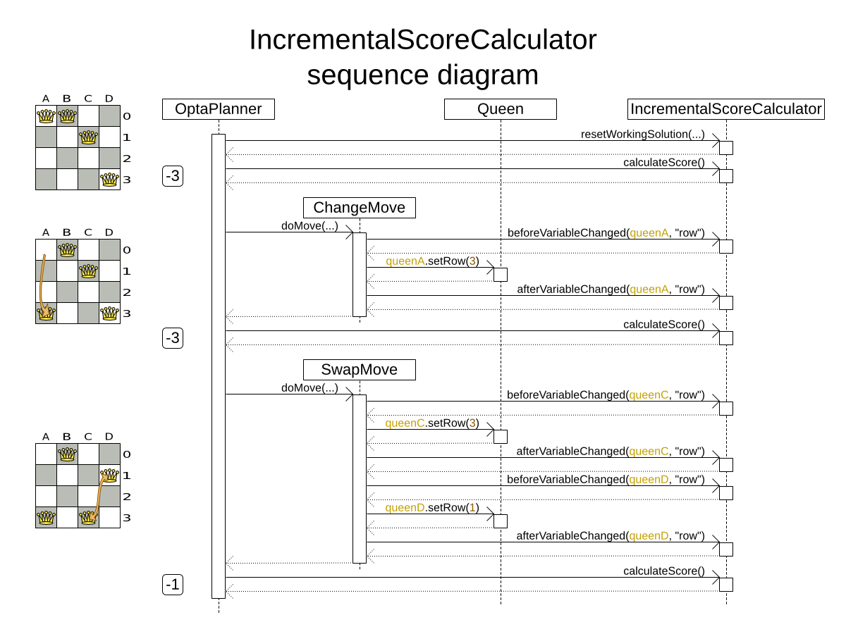
For example in n queens:
public class NQueensAdvancedIncrementalScoreCalculator extends AbstractIncrementalScoreCalculator<NQueens> {
private Map<Integer, List<Queen>> rowIndexMap;
private Map<Integer, List<Queen>> ascendingDiagonalIndexMap;
private Map<Integer, List<Queen>> descendingDiagonalIndexMap;
private int score;
public void resetWorkingSolution(NQueens nQueens) {
int n = nQueens.getN();
rowIndexMap = new HashMap<Integer, List<Queen>>(n);
ascendingDiagonalIndexMap = new HashMap<Integer, List<Queen>>(n * 2);
descendingDiagonalIndexMap = new HashMap<Integer, List<Queen>>(n * 2);
for (int i = 0; i < n; i++) {
rowIndexMap.put(i, new ArrayList<Queen>(n));
ascendingDiagonalIndexMap.put(i, new ArrayList<Queen>(n));
descendingDiagonalIndexMap.put(i, new ArrayList<Queen>(n));
if (i != 0) {
ascendingDiagonalIndexMap.put(n - 1 + i, new ArrayList<Queen>(n));
descendingDiagonalIndexMap.put((-i), new ArrayList<Queen>(n));
}
}
score = 0;
for (Queen queen : nQueens.getQueenList()) {
insert(queen);
}
}
public void beforeEntityAdded(Object entity) {
// Do nothing
}
public void afterEntityAdded(Object entity) {
insert((Queen) entity);
}
public void beforeVariableChanged(Object entity, String variableName) {
retract((Queen) entity);
}
public void afterVariableChanged(Object entity, String variableName) {
insert((Queen) entity);
}
public void beforeEntityRemoved(Object entity) {
retract((Queen) entity);
}
public void afterEntityRemoved(Object entity) {
// Do nothing
}
private void insert(Queen queen) {
Row row = queen.getRow();
if (row != null) {
int rowIndex = queen.getRowIndex();
List<Queen> rowIndexList = rowIndexMap.get(rowIndex);
score -= rowIndexList.size();
rowIndexList.add(queen);
List<Queen> ascendingDiagonalIndexList = ascendingDiagonalIndexMap.get(queen.getAscendingDiagonalIndex());
score -= ascendingDiagonalIndexList.size();
ascendingDiagonalIndexList.add(queen);
List<Queen> descendingDiagonalIndexList = descendingDiagonalIndexMap.get(queen.getDescendingDiagonalIndex());
score -= descendingDiagonalIndexList.size();
descendingDiagonalIndexList.add(queen);
}
}
private void retract(Queen queen) {
Row row = queen.getRow();
if (row != null) {
List<Queen> rowIndexList = rowIndexMap.get(queen.getRowIndex());
rowIndexList.remove(queen);
score += rowIndexList.size();
List<Queen> ascendingDiagonalIndexList = ascendingDiagonalIndexMap.get(queen.getAscendingDiagonalIndex());
ascendingDiagonalIndexList.remove(queen);
score += ascendingDiagonalIndexList.size();
List<Queen> descendingDiagonalIndexList = descendingDiagonalIndexMap.get(queen.getDescendingDiagonalIndex());
descendingDiagonalIndexList.remove(queen);
score += descendingDiagonalIndexList.size();
}
}
public SimpleScore calculateScore() {
return SimpleScore.valueOf(score);
}
}Configure it in your solver configuration:
<scoreDirectorFactory>
<scoreDefinitionType>...</scoreDefinitionType>
<incrementalScoreCalculatorClass>org.optaplanner.examples.nqueens.solver.score.NQueensAdvancedIncrementalScoreCalculator</incrementalScoreCalculatorClass>
</scoreDirectorFactory>Optionally, to explain a score with ScoreDirector.getConstraintMatchTotals() or to get
better output when the IncrementalScoreCalculator is corrupted in
FAST_ASSERT or FULL_ASSERT environmentMode, implement also the
ConstraintMatchAwareIncrementalScoreCalculator interface:
public interface ConstraintMatchAwareIncrementalScoreCalculator<Sol extends Solution> {
void resetWorkingSolution(Sol workingSolution, boolean constraintMatchEnabled);
Collection<ConstraintMatchTotal> getConstraintMatchTotals();
}Implement your score calculation using the Drools rule engine. Every score constraint is written as one or more score rules.
Advantages:
Incremental score calculation for free
Because most DRL syntax uses forward chaining, it does incremental calculation without any extra code
Score constraints are isolated as separate rules
Easy to add or edit existing score rules
Flexibility to augment your score constraints by
Defining them in decision tables
Excel (XLS) spreadsheet
KIE Workbench WebUI
Translate them into natural language with DSL
Store and release in the KIE Workbench repository
Performance optimizations in future versions for free
In every release, the Drools rule engine tends to become faster
Disadvantages:
DRL learning curve
Usage of DRL
Polyglot fear can prohibit the use of a new language such as DRL in some organizations
There are several ways to define where your score rules live.
This is the easy way: the score rule live in a DRL file which is provided as a classpath resource. Just
add the score rules DRL file in the solver configuration as a <scoreDrl>
element:
<scoreDirectorFactory>
<scoreDefinitionType>...</scoreDefinitionType>
<scoreDrl>org/optaplanner/examples/nqueens/solver/nQueensScoreRules.drl</scoreDrl>
</scoreDirectorFactory>In a typical project (following the Maven directory structure), that DRL file would be located at
$PROJECT_DIR/src/main/resources/org/optaplanner/examples/nqueens/solver/nQueensScoreRules.drl
(even for a war project).
Note
The <scoreDrl> element expects a classpath resource, as defined by
ClassLoader.getResource(String), it does not accept a File, nor an
URL, nor a webapp resource. See below to use a File instead.
Add multiple <scoreDrl> elements if the score rules are split across multiple
DRL files.
Optionally, you can also set drools configuration properties (but be careful of backwards compatibility issues):
<scoreDirectorFactory>
...
<scoreDrl>org/optaplanner/examples/nqueens/solver/nQueensScoreRules.drl</scoreDrl>
<kieBaseConfigurationProperties>
<drools.equalityBehavior>...</drools.equalityBehavior>
</kieBaseConfigurationProperties>
</scoreDirectorFactory>To use File on the local file system, instead of a classpath resource, add the score
rules DRL file in the solver configuration as a <scoreDrlFile> element:
<scoreDirectorFactory>
<scoreDefinitionType>...</scoreDefinitionType>
<scoreDrlFile>/home/ge0ffrey/tmp/nQueensScoreRules.drl</scoreDrlFile>
</scoreDirectorFactory>Warning
For portability reasons, a classpath resource is recommended over a File. An application build on one computer, but used on another computer, might not find the file on the same location. Worse, if they use a different Operating System, it's hard to choose a portable file path.
Add multiple <scoreDrlFile> elements if the score rules are split across
multiple DRL files.
To build the KieBase yourself or to combine Planner with KIE Workbench (formerly
known as Guvnor), set the KieBase on the SolverFactory before building
the Solver:
solverFactory.getSolverConfig().getScoreDirectorFactoryConfig.setKieBase(kieBase);Note
To be able to define your score rules in Drools Workbench, you'll want to:
Upload the
optaplanner-corejar as a POJO model.Add a global variable called
scoreHolder(see below).
Here's an example of a score constraint implemented as a score rule in a DRL file:
rule "multipleQueensHorizontal"
when
Queen($id : id, row != null, $i : rowIndex)
Queen(id > $id, rowIndex == $i)
then
scoreHolder.addConstraintMatch(kcontext, -1);
endThis score rule will fire once for every 2 queens with the same rowIndex. The
(id > $id) condition is needed to assure that for 2 queens A and B, it can only fire for
(A, B) and not for (B, A), (A, A) or (B, B). Let's take a closer look at this score rule on this solution of 4
queens:
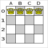
In this solution the multipleQueensHorizontal score rule will fire for 6 queen couples: (A, B), (A, C),
(A, D), (B, C), (B, D) and (C, D). Because none of the queens are on the same vertical or diagonal line, this
solution will have a score of -6. An optimal solution of 4 queens has a score of
0.
Note
Notice that every score rule will relate to at least 1 planning entity class (directly or indirectly through a logically inserted fact).
This is normal: it would be a waste of time to write a score rule that only relates to problem facts, as the consequence will never change during planning, no matter what the possible solution.
Note
The kcontext variable is a magic variable in Drools Expert. The
scoreHolder's method uses it to do incremental score calculation correctly and to create a
ConstraintMatch instance.
A ScoreHolder instance is asserted into the KieSession as a global
called scoreHolder. Your score rules need to (directly or indirectly) update that
instance.
global SimpleScoreHolder scoreHolder;
rule "multipleQueensHorizontal"
when
Queen($id : id, row != null, $i : rowIndex)
Queen(id > $id, rowIndex == $i)
then
scoreHolder.addConstraintMatch(kcontext, -1);
end
// multipleQueensVertical is obsolete because it is always 0
rule "multipleQueensAscendingDiagonal"
when
Queen($id : id, row != null, $i : ascendingDiagonalIndex)
Queen(id > $id, ascendingDiagonalIndex == $i)
then
scoreHolder.addConstraintMatch(kcontext, -1);
end
rule "multipleQueensDescendingDiagonal"
when
Queen($id : id, row != null, $i : descendingDiagonalIndex)
Queen(id > $id, descendingDiagonalIndex == $i)
then
scoreHolder.addConstraintMatch(kcontext, -1);
endMost use cases will also weigh their constraint types or even their matches differently, by using a specific weight for each constraint match.
Here's an example from CurriculumCourse, where assigning a Lecture to a
Room which is missing 2 seats is weighted equally bad as having 1 isolated
Lecture in a Curriculum:
global HardSoftScoreHolder scoreHolder;
// RoomCapacity: For each lecture, the number of students that attend the course must be less or equal
// than the number of seats of all the rooms that host its lectures.
// Each student above the capacity counts as 1 point of penalty.
rule "roomCapacity"
when
$room : Room($capacity : capacity)
$lecture : Lecture(room == $room, studentSize > $capacity, $studentSize : studentSize)
then
scoreHolder.addSoftConstraintMatch(kcontext, ($capacity - $studentSize));
end
// CurriculumCompactness: Lectures belonging to a curriculum should be adjacent
// to each other (i.e., in consecutive periods).
// For a given curriculum we account for a violation every time there is one lecture not adjacent
// to any other lecture within the same day.
// Each isolated lecture in a curriculum counts as 2 points of penalty.
rule "curriculumCompactness"
when
...
then
scoreHolder.addSoftConstraintMatch(kcontext, -2);
endThe InitializingScoreTrend specifies how the Score will change as more and more variables
are initialized (while the already initialized variables don't change). Some optimization algorithms (such
Construction Heuristics and Exhaustive Search) run faster if they have such information.
For for the Score (or each score level separately), specify a trend:
ANY(default): Initializing an extra variable can change the score positively or negatively. Gives no performance gain.ONLY_UP(rare): Initializing an extra variable can only change the score positively. Implies that:There are only positive constraints
And initializing the next variable can not unmatch a positive constraint that was matched by a previous initialized variable.
ONLY_DOWN: Initializing an extra variable can only change the score negatively. Implies that:There are only negative constraints
And initializing the next variable can not unmatch a negative constraint that was matched by a previous initialized variable.
Most use cases only have negative constraints. Many of those have an
InitializingScoreTrend that only goes down:
<scoreDirectorFactory>
<scoreDefinitionType>HARD_SOFT</scoreDefinitionType>
<scoreDrl>.../cloudBalancingScoreRules.drl</scoreDrl>
<initializingScoreTrend>ONLY_DOWN</initializingScoreTrend>
</scoreDirectorFactory>Alternatively, you can also specify the trend for each score level separately:
<scoreDirectorFactory>
<scoreDefinitionType>HARD_SOFT</scoreDefinitionType>
<scoreDrl>.../cloudBalancingScoreRules.drl</scoreDrl>
<initializingScoreTrend>ONLY_DOWN/ONLY_DOWN</initializingScoreTrend>
</scoreDirectorFactory>Put the environmentMode in FULL_ASSERT (or
FAST_ASSERT) to detect corruption in the incremental score calculation. For more information, see the section about environmentMode. However, that will not
verify that your score calculator implements your score constraints as your business actually desires.
A piece of incremental score calculator code can be difficult to write and to review. Assert its correctness
by using a different implementation (for example a EasyScoreCalculator) to do the assertions
triggered by the environmentMode. Just configure the different implementation as a
assertionScoreDirectorFactory:
<environmentMode>FAST_ASSERT</environmentMode>
...
<scoreDirectorFactory>
<scoreDefinitionType>...</scoreDefinitionType>
<scoreDrl>org/optaplanner/examples/nqueens/solver/nQueensScoreRules.drl</scoreDrl>
<assertionScoreDirectorFactory>
<easyScoreCalculatorClass>org.optaplanner.examples.nqueens.solver.score.NQueensEasyScoreCalculator</easyScoreCalculatorClass>
</assertionScoreDirectorFactory>
</scoreDirectorFactory>This way, the scoreDrl will be validated by the
EasyScoreCalculator.
The Solver will normally spend most of its execution time running the score calculation
(which is called in its deepest loops). Faster score calculation will return the same solution in less time with
the same algorithm, which normally means a better solution in equal time.
After solving a problem, the Solver will log the average calculation count per
second. This is a good measurement of Score calculation performance, despite that it is affected by non
score calculation execution time. It depends on the problem scale of the problem dataset. Normally, even for high
scale problems, it is higher than 1000, except when you're using
EasyScoreCalculator.
Important
When improving your score calculation, focus on maximizing the average calculation count per second, instead of maximizing the best score. A big improvement in score calculation can sometimes yield little or no best score improvement, for example when the algorithm is stuck in a local or global optima. If you're watching the calculation count instead, score calculation improvements are far more visible.
Furthermore, watching the calculation count, allows you to remove or add score constraints, and still compare it with the original calculation count. Comparing the best score with the original would be wrong, because it's comparing apples and oranges.
When a Solution changes, incremental score calculation (AKA delta based score
calculation), will calculate the delta with the previous state to find the new Score, instead
of recalculating the entire score on every solution evaluation.
For example, if a single queen A moves from row 1 to 2, it won't
bother to check if queen B and C can attack each other, since neither of them changed.
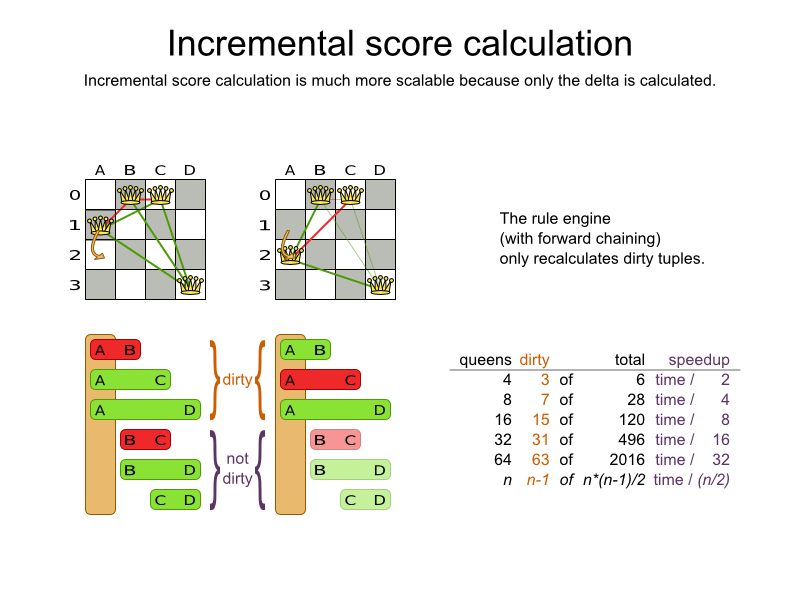
This is a huge performance and scalability gain. Drools score calculation gives you this huge scalability gain without forcing you to write a complicated incremental score calculation algorithm. Just let the Drools rule engine do the hard work.
Notice that the speedup is relative to the size of your planning problem (your n), making incremental score calculation far more scalable.
Do not call remote services in your score calculation (except if you're bridging
EasyScoreCalculator to a legacy system). The network latency will kill your score calculation
performance. Cache the results of those remote services if possible.
If some parts of a constraint can be calculated once, when the Solver starts, and never
change during solving, then turn them into cached problem facts.
If you know a certain constraint can never be broken (or it is always broken), don't bother writing a score
constraint for it. For example in n queens, the score calculation doesn't check if multiple queens occupy the same
column, because a Queen's column never changes and every
Solution starts with each Queen on a different
column.
Note
Don't go overboard with this. If some datasets don't use a specific constraint but others do, just return out of the constraint as soon as you can. There is no need to dynamically change your score calculation based on the dataset.
Instead of implementing a hard constraint, it can sometimes be built in. For example: If
Lecture A should never be assigned to Room X, but it uses
ValueRangeProvider on Solution, so the Solver will often try to assign it to
Room X too (only to find out that it breaks a hard constraint). Use a ValueRangeProvider on the planning entity or filtered selection to define that Course A should only be assigned a
Room different than X.
This can give a good performance gain in some use cases, not just because the score calculation is faster, but mainly because most optimization algorithms will spend less time evaluating unfeasible solutions. However, usually this not a good idea because there is a real risk of trading short term benefits for long term harm:
Many optimization algorithms rely on the freedom to break hard constraints when changing planning entities, to get out of local optima.
Both implementation approaches have limitations (feature compatiblity, disabling automatic performance optimizations, ...), as explained in their documentation.
Verify that your score calculation happens in the correct
Numbertype. If you're making the sum ofintvalues, don't let Drools sum it in adoublewhich takes longer.For optimal performance, always use server mode (
java -server). We have seen performance increases of 50% by turning on server mode.For optimal performance, use the latest Java version. For example, in the past we have seen performance increases of 30% by switching from java 1.5 to 1.6.
Always remember that premature optimization is the root of all evil. Make sure your design is flexible enough to allow configuration based tweaking.
Make sure that none of your score constraints cause a score trap. A trapped score constraint uses the same weight for different constraint matches, when it could just as easily use a different weight. It effectively lumps its constraint matches together, which creates a flatlined score function for that constraint. This can cause a solution state in which several moves need to be done to resolve or lower the weight of that single constraint. Some examples of score traps:
If you need 2 doctors at each table, but you're only moving 1 doctor at a time. So the solver has no incentive to move a doctor to a table with no doctors. Punish a table with no doctors more then a table with only 1 doctor in that score constraint in the score function.
2 exams need to be conducted at the same time, but you're only moving 1 exam at a time. So the solver has to move one of those exams to another timeslot without moving the other in the same move. Add a coarse-grained move that moves both exams at the same time.
For example, consider this score trap. If the blue item moves from an overloaded computer to an empty computer, the hard score should improve. The trapped score implementation fails to do that:
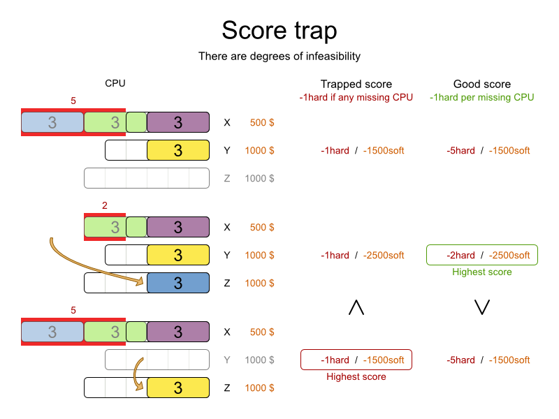
The Solver should eventually get out of this trap, but it will take a lot of effort (especially if there are even more processes on the overloaded computer). Before they do that, they might actually start moving more processes into that overloaded computer, as there is no penalty for doing so.
Note
Avoiding score traps does not mean that your score function should be smart enough to avoid local optima. Leave it to the optimization algorithms to deal with the local optima.
Avoiding score traps means to avoid - for each score constraint individually - a flatlined score function.
Important
Always specify the degree of infeasibility. The business will often say: "if the solution is infeasible, it doesn't matter how infeasible it." While that's true for the business, it's not true for score calculation: it benefits from knowing how infeasible it is. In practice, soft constraints usually do this naturally and it's just a matter of doing it for the hard constraints too.
There are several ways to deal with a score trap:
Improve the score constraint to make a distinction in the score weight. For example: penalize
-1hardfor every missing CPU, instead of just-1hardif any CPU is missing.If changing the score constraint is not allowed from the business perspective, add a lower score level with a score constraint that makes such a distinction. For example: penalize
-1subsoftfor every missing CPU, on top of-1hardif any CPU is missing. The business ignores the subsoft score level.Add coarse-grained moves and union select them with the existing fine-grained moves. A coarse-grained move effectively does multiple moves to directly get out of a score trap with a single move. For example: move multiple items from the same container to another container.
Not all score constraints have the same performance cost. Sometimes 1 score constraint can kill the score calculation performance outright. Use the Benchmarker to do a 1 minute run and check what happens to the average calculation count per second if you comment out all but 1 of the score constraints.
Some use cases have a business requirement to provide a fair schedule (usually as a soft score constraint), for example:
Fairly distribute the workload amongst the employees, to avoid envy.
Evenly distribute the workload amongst assets, to improve reliability.
Implementing such a constraint can seem difficult (especially because there are different ways to formalize
fairness), but usually the squared workload implementation behaves most desirable: for each
employee/asset, count the workload w and subtract w² from the score.
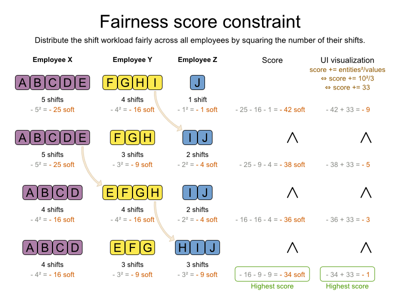
As shown above, the squared workload implementation guarantees that if you select 2 employees from a given solution and make their distribution between those 2 employees fairer, then the resulting new solution will have a better overall score. Don't just use the difference from the average workload, as that can lead to unfairness, as demonstrated below.
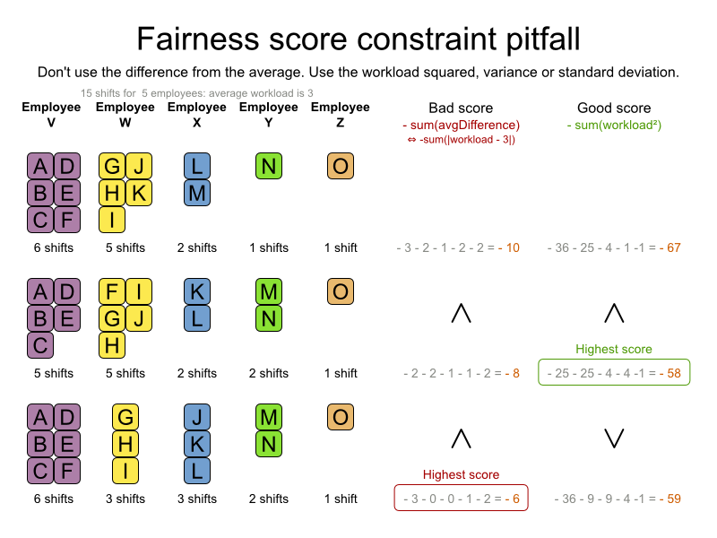
Note
Instead of the squared workload, it's also possible to use the variance (squared difference to the average) or the standard deviation (square root of the variance). This has no effect on the score comparison, because the average won't change during planning. It's just more work to implement (because the average needs to be known) and trivially slower (because the calculation is a bit longer).
When the workload is perfect balanced, the user often likes to see a 0 score, instead of
the distracting -34soft in the image above (for the last solution which is almost perfectly
balanced). To nullify this, either add the average multiplied by the number of entities to the score or instead
show the variance or standard deviation in the UI.
Other parts of your application, for example your webUI, might need to calculate the score too. Do that by
reusing the ScoreDirectorFactory of the Solver to build a separate
ScoreDirector for that webUI:
ScoreDirectorFactory scoreDirectorFactory = solver.getScoreDirectorFactory();
ScoreDirector guiScoreDirector = scoreDirectorFactory.buildScoreDirector();Then use it when you need to calculate the Score of a Solution:
guiScoreDirector.setWorkingSolution(solution);
Score score = guiScoreDirector.calculateScore();To explain in the GUI what entities are causing which part of the Score, get the
ConstraintMatch objects from the ScoreDirector:
for (ConstraintMatchTotal constraintMatchTotal : guiScoreDirector.getConstraintMatchTotals()) {
String constraintName = constraintMatchTotal.getConstraintName();
Number weightTotal = constraintMatchTotal.getWeightTotalAsNumber();
for (ConstraintMatch constraintMatch : constraintMatchTotal.getConstraintMatchSet()) {
List<Object> justificationList = constraintMatch.getJustificationList();
Number weight = constraintMatch.getWeightAsNumber();
...
}
}Note
Drools score calculation supports constraint matches automatically, but incremental Java score calculation requires requires implementing an extra interface (see that section).
- 6.1. Search Space Size in the Real World
- 6.2. Does Planner Find the Optimal Solution?
- 6.3. Architecture Overview
- 6.4. Optimization Algorithms Overview
- 6.5. Which Optimization Algorithms Should I Use?
- 6.6. Power tweaking or default parameter values
- 6.7. Solver Phase
- 6.8. Scope Overview
- 6.9. Termination
- 6.10. SolverEventListener
- 6.11. Custom Solver Phase
The number of possible solutions for a planning problem can be mind blowing. For example:
4 queens has
256possible solutions (4^4) and 2 optimal solutions.5 queens has
3125possible solutions (5^5) and 1 optimal solution.8 queens has
16777216possible solutions (8^8) and 92 optimal solutions.64 queens has more than
10^115possible solutions (64^64).Most real-life planning problems have an incredible number of possible solutions and only 1 or a few optimal solutions.
For comparison: the minimal number of atoms in the known universe (10^80). As a planning problem gets bigger, the search space tends to blow up really fast. Adding only 1 extra planning entity or planning value can heavily multiply the running time of some algorithms.
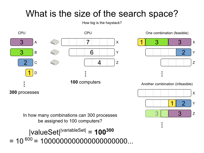
Calculating the number of possible solutions depends on the design of the domain model:
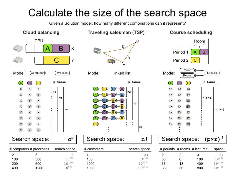
Note
This search space size calculation includes infeasible solutions (if they can be represented by the model), because:
The optimal solution might be infeasible.
There are many types of hard constraints which cannot be incorporated in the formula practically. For example in Cloud Balancing, try incorporating the CPU capacity constraint in the formula.
Even in cases were adding some of the hard constraints in the formula is practical, for example Course Scheduling, the resulting search space is still huge.
An algorithm that checks every possible solution (even with pruning such as in Branch And Bound) can easily run for billions of years on a single real-life planning problem. What we really want is to find the best solution in the limited time at our disposal. Planning competitions (such as the International Timetabling Competition) show that Local Search variations (Tabu Search, Simulated Annealing, Late Acceptance, ...) usually perform best for real-world problems given real-world time limitations.
The business wants the optimal solution, but they also have other requirements:
Scale out: Large production datasets must not crash and have good results too.
Optimize the right problem: The constraints must match the actual business needs.
Available time: The solution must be found in time, before it becomes useless to execute.
Reliability: Every dataset must have at least a decent result (better than a human planner).
Given these requirements, and despite the promises of some salesmen, it's usually impossible for anyone or anything to find the optimal solution. Therefore, Planner focuses on finding the best solution in available time. In realistic, independent competitions, it often comes out as the best reusable software.
The nature of NP-complete problems make scaling a prime concern. The result quality of a small dataset guarantees nothing about the result quality of a large dataset. Scaling issues cannot be mitigated by hardware purchases later on. Start testing with a production sized dataset as soon as possible. Don't assess quality on small datasets (unless production encounters only such datasets). Instead, solve a production sized dataset and compare the results of longer executions, different algorithms and - if available - the human planner.
Planner is the first framework to combine optimization algorithms (metaheuristics, ...) with score calculation by a rule engine (such as Drools Expert). This combination turns out to be a very efficient, because:
A rule engine such as Drools Expert is great for calculating the score of a solution of a planning problem. It makes it easy and scalable to add additional soft or hard constraints such as "a teacher shouldn't teach more then 7 hours a day". It does delta based score calculation without any extra code. However it tends to be not suitable to actually find new solutions.
An optimization algorithm is great at finding new improving solutions for a planning problem, without necessarily brute-forcing every possibility. However it needs to know the score of a solution and offers no support in calculating that score efficiently.
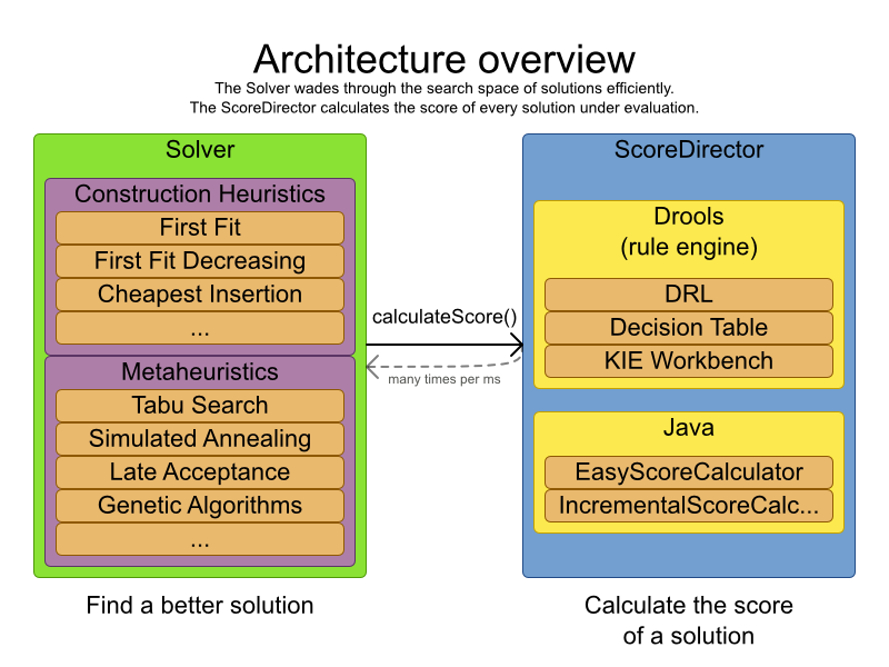
Planner supports 3 families of optimization algorithms: Exhaustive Search, Construction Heuristics and Metaheuristics. In practice, Metaheuristics (in combination with Construction Heuristics to initialize) are the recommended choice:
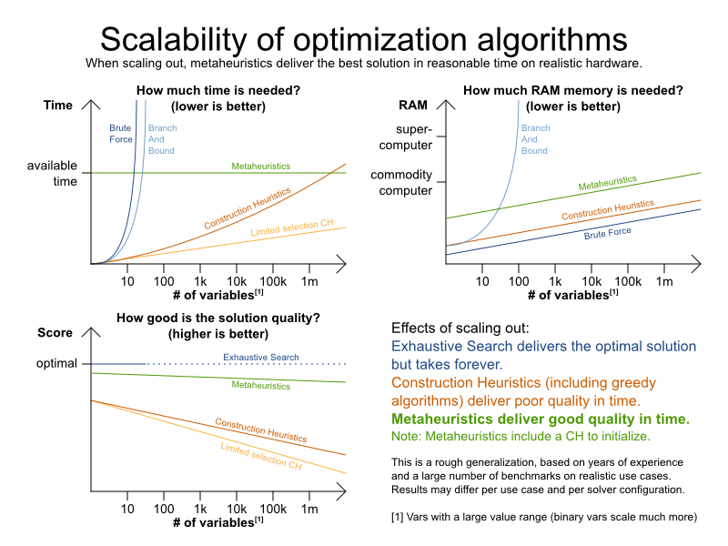
Each of these families of algorithms has multiple optimization algorithms:
Table 6.1. Optimization Algorithms Overview
| Algorithm | Scalable? | Optimal? | Easy to use? | Tweakable? | Requires CH? |
|---|---|---|---|---|---|
| Exhaustive Search (ES) | |||||
| Brute Force | 0/5 | 5/5 | 5/5 | 0/5 | No |
| Branch And Bound | 0/5 | 5/5 | 4/5 | 2/5 | No |
| Construction heuristics (CH) | |||||
| First Fit | 5/5 | 1/5 | 5/5 | 1/5 | No |
| First Fit Decreasing | 5/5 | 2/5 | 4/5 | 2/5 | No |
| Weakest Fit | 5/5 | 2/5 | 4/5 | 2/5 | No |
| Weakest Fit Decreasing | 5/5 | 2/5 | 4/5 | 2/5 | No |
| Strongest Fit | 5/5 | 2/5 | 4/5 | 2/5 | No |
| Strongest Fit Decreasing | 5/5 | 2/5 | 4/5 | 2/5 | No |
| Cheapest Insertion | 3/5 | 2/5 | 5/5 | 2/5 | No |
| Regret Insertion | 3/5 | 2/5 | 5/5 | 2/5 | No |
| Metaheuristics (MH) | |||||
| Local Search | |||||
| Hill Climbing | 5/5 | 2/5 | 4/5 | 3/5 | Yes |
| Tabu Search | 5/5 | 4/5 | 3/5 | 5/5 | Yes |
| Simulated Annealing | 5/5 | 4/5 | 2/5 | 5/5 | Yes |
| Late Acceptance | 5/5 | 4/5 | 3/5 | 5/5 | Yes |
| Step Counting Hill Climbing | 5/5 | 4/5 | 3/5 | 5/5 | Yes |
| Evolutionary Algorithms | |||||
| Evolutionary Strategies | 4/5 | 3/5 | 2/5 | 5/5 | Yes |
| Genetic Algorithms | 4/5 | 3/5 | 2/5 | 5/5 | Yes |
If you want to learn more about metaheuristics, read the free books Essentials of Metaheuristics or Clever Algorithms.
The best optimization algorithms configuration for your use case depends heavily on your use case. Nevertheless, this vanilla recipe will get you into the game with a pretty good configuration, probably much better than what you're used to.
Start with a quick configuration that involves little or no configuration and optimization code:
Next, implement planning entity difficulty comparison and turn it into:
Next, add Late Acceptance behind it:
First Fit Decreasing
Late Acceptance. A Late Acceptance size of 400 usually works well.
At this point the free lunch is over. The return on invested time lowers. The result is probably already more than good enough.
But you can do even better, at a lower return on invested time. Use the Benchmarker and try a couple of different Tabu Search, Simulated Annealing and Late Acceptance configurations, for example:
First Fit Decreasing
Tabu Search. An entity tabu size of 7 usually works well.
Use the Benchmarker to improve the values for those size parameters.
If it's worth your time, continue experimenting further. For example, try combining multiple algorithms together:
First Fit Decreasing
Late Acceptance (relatively long time)
Tabu Search (relatively short time)
Many optimization algorithms have parameters which affect results and scalability. Planner applies configuration by exception, so all optimization algorithms have default parameter values. This is very similar to the Garbage Collection parameters in a JVM: most users have no need to tweak them, but power users do tweak them.
The default parameter values are good enough for many cases (and especially for prototypes), but if development time allows, it can be well worth to power tweak them with the benchmarker for better results and scalability on a specific use case. The documentation for each optimization algorithm also declares its advanced configuration for power tweaking.
Warning
The default value of parameters will change between minor versions, to improve them for most users (but not necessary for you). To shield yourself from these changes, for better or worse, always use the advanced configuration. This is not recommended.
A Solver can use multiple optimization algorithms in sequence. Each
optimization algorithm is represented by a solver Phase. There is never more than 1
Phase solving at the same time.
Note
Some Phase implementations can combine techniques from multiple optimization algorithms,
but it is still just 1 Phase. For example: a Local Search Phase can do
Simulated Annealing with entity Tabu.
Here's a configuration that runs 3 phases in sequence:
<solver>
...
<constructionHeuristic>
... <!-- First phase: First Fit Decreasing -->
</constructionHeuristic>
<localSearch>
... <!-- Second phase: Late Acceptance -->
</localSearch>
<localSearch>
... <!-- Third phase: Tabu Search -->
</localSearch>
</solver>The solver phases are run in the order defined by solver configuration. When the first
Phase terminates, the second Phase starts, and so on. When the last
Phase terminates, the Solver terminates. Usually, a Solver
will first run a construction heuristic and then run 1 or multiple metaheuristics:
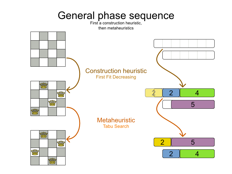
If no phases are configured, Planner will default to a Construction Heuristic phase followed by a Local Search phase.
Some phases (especially construction heuristics) will terminate automatically. Other phases (especially
metaheuristics) will only terminate if the Phase is configured to terminate:
<solver>
...
<termination><!-- Solver termination -->
<secondsSpentLimit>90</secondsSpentLimit>
</termination>
<localSearch>
<termination><!-- Phase termination -->
<secondsSpentLimit>60</secondsSpentLimit><!-- Give the next phase a chance to run too, before the Solver terminates -->
</termination>
...
</localSearch>
<localSearch>
...
</localSearch>
</solver>If the Solver terminates (before the last Phase terminates itself), the
current phase is terminated and all subsequent phases won't run.
A solver will iteratively run phases. Each phase will usually iteratively run steps. Each step, in turn, usually iteratively runs moves. These form 4 nested scopes: solver, phase, step and move.
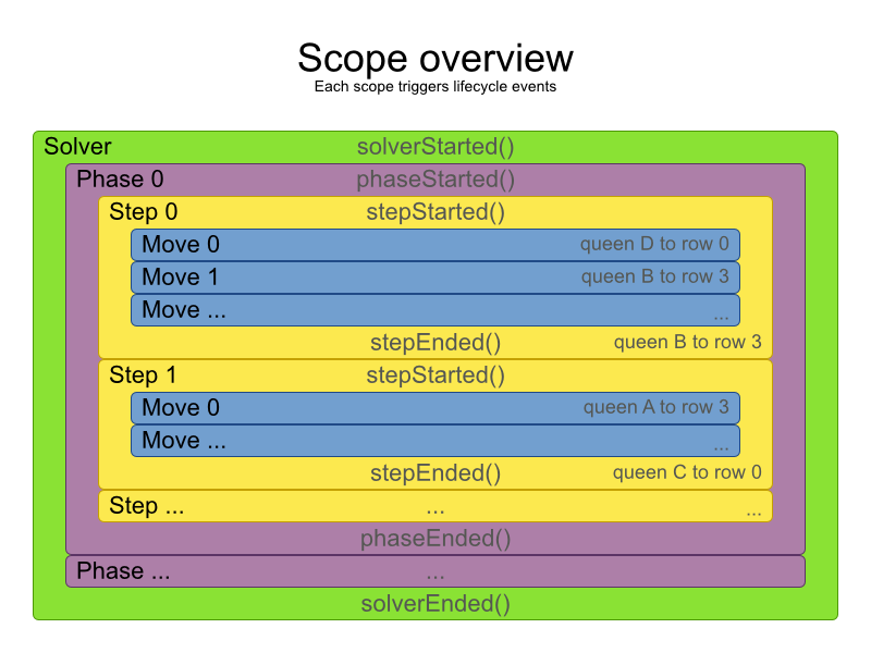
Configure logging to display the log messages of each scope.
Not all phases terminate automatically and sometimes you don't want to wait that long anyway. A
Solver can be terminated synchronously by up-front configuration or asynchronously from another
thread.
Especially metaheuristic phases will need to be told when to stop solving. This can be because of a number of reasons: the time is up, the perfect score has been reached, ... The only thing you can't depend on, is on finding the optimal solution (unless you know the optimal score), because a metaheuristic algorithm generally doesn't know it when it finds the optimal solution. For real-life problems this doesn't turn out to be much of a problem, because finding the optimal solution could take years, so you'll want to terminate sooner anyway. The only thing that matters is finding the best solution in the available time.
For synchronous termination, configure a Termination on a Solver or a
Phase when it needs to stop. You can implement your own Termination, but the
built-in implementations should suffice for most needs. Every Termination can calculate a
time gradient (needed for some optimization algorithms), which is a ratio between the time
already spent solving and the estimated entire solving time of the Solver or
Phase.
Terminates when an amount of time has been used:
<termination>
<millisecondsSpentLimit>500</millisecondsSpentLimit>
</termination> <termination>
<secondsSpentLimit>10</secondsSpentLimit>
</termination> <termination>
<minutesSpentLimit>5</minutesSpentLimit>
</termination> <termination>
<hoursSpentLimit>1</hoursSpentLimit>
</termination>Note
This Termination will most likely sacrifice perfect reproducibility (even with
environmentMode REPRODUCIBLE) because the available CPU time differs
frequently between runs:
The available CPU time influences the number of steps that can be taken, which might be a few more or less.
The
Terminationmight produce slightly different time gradient values, which will send time gradient based algorithms (such as Simulated Annealing) on a radically different path.
Terminates when the best score hasn't improved in an amount of time:
<localSearch>
<termination>
<unimprovedMillisecondsSpentLimit>500</unimprovedMillisecondsSpentLimit>
</termination>
</localSearch> <localSearch>
<termination>
<unimprovedSecondsSpentLimit>10</unimprovedSecondsSpentLimit>
</termination>
</localSearch> <localSearch>
<termination>
<unimprovedMinutesSpentLimit>5</unimprovedMinutesSpentLimit>
</termination>
</localSearch> <localSearch>
<termination>
<unimprovedHoursSpentLimit>1</unimprovedHoursSpentLimit>
</termination>
</localSearch>This termination should not be applied to Construction Heuristics, because they only update the best
solution at the end. Therefore it might be better to configure it on a specific Phase (such as
<localSearch>), instead of on the Solver itself.
Note
This Termination will most likely sacrifice perfect reproducibility (even with
environmentMode REPRODUCIBLE) because the available CPU time differs
frequently between runs:
The available CPU time influences the number of steps that can be taken, which might be a few more or less.
The
Terminationmight produce slightly different time gradient values, which will send time gradient based algorithms (such as Simulated Annealing) on a radically different path.
Terminates when a certain score has been reached. You can use this Termination if you
know the perfect score, for example for 4 queens (which uses a SimpleScore):
<termination>
<bestScoreLimit>0</bestScoreLimit>
</termination>For a planning problem with a HardSoftScore, it could look like this:
<termination>
<bestScoreLimit>0hard/-5000soft</bestScoreLimit>
</termination>For a planning problem with a BendableScore with 3 hard levels and 1 soft level, it could look like this:
<termination>
<bestScoreLimit>0/0/0/-5000</bestScoreLimit>
</termination>To terminate once a feasible solution has been reached, this Termination isn't practical
because it requires a bestScoreLimit such as 0hard/-2147483648soft. Instead,
use the next termination.
Terminates when a certain score is feasible. Requires that the Score implementation
implements FeasibilityScore.
<termination>
<bestScoreFeasible>true</bestScoreFeasible>
</termination>This Termination is usually combined with other terminations.
Terminates when an amount of steps has been reached:
<localSearch>
<termination>
<stepCountLimit>100</stepCountLimit>
</termination>
</localSearch>This Termination can only be used for a Phase (such as
<localSearch>), not for the Solver itself.
Terminates when the best score hasn't improved in a number of steps:
<localSearch>
<termination>
<unimprovedStepCountLimit>100</unimprovedStepCountLimit>
</termination>
</localSearch>If the score hasn't improved recently, it's probably not going to improve soon anyway and it's not worth the effort to continue. We have observed that once a new best solution is found (even after a long time of no improvement on the best solution), the next few steps tend to improve the best solution too.
This Termination can only be used for a Phase (such as
<localSearch>), not for the Solver itself.
Terminations can be combined, for example: terminate after 100 steps or if a score of
0 has been reached:
<termination>
<terminationCompositionStyle>OR</terminationCompositionStyle>
<stepCountLimit>100</stepCountLimit>
<bestScoreLimit>0</bestScoreLimit>
</termination>Alternatively you can use AND, for example: terminate after reaching a feasible score of at least
-100 and no improvements in 5 steps:
<termination>
<terminationCompositionStyle>AND</terminationCompositionStyle>
<unimprovedStepCountLimit>5</unimprovedStepCountLimit>
<bestScoreLimit>-100</bestScoreLimit>
</termination>This example ensures it doesn't just terminate after finding a feasible solution, but also completes any obvious improvements on that solution before terminating.
Sometimes you'll want to terminate a Solver early from another thread, for example because a user action or
a server restart. This cannot be configured by a Termination as it's impossible to predict when
and if it will occur. Therefore the Solver interface has these 2 thread-safe methods:
public interface Solver {
// ...
boolean terminateEarly();
boolean isTerminateEarly();
}If you call the terminateEarly() method from another thread, the
Solver will terminate at its earliest convenience and the solve(Solution)
method will return in the original Solver thread.
Each time a new best solution is found, the Solver fires a
BestSolutionChangedEvent, in the solver's thread.
To listen to such events, add a SolverEventListener to the
Solver:
public interface Solver {
// ...
void addEventListener(SolverEventListener<? extends Solution> eventListener);
void removeEventListener(SolverEventListener<? extends Solution> eventListener);
}The BestSolutionChangedEvent's newBestSolution might not be initialized
or feasible. Use the methods on BestSolutionChangedEvent to detect such cases:
solver.addEventListener(new SolverEventListener<CloudBalance>() {
public void bestSolutionChanged(BestSolutionChangedEvent<CloudBalance> event) {
// Ignore invalid solutions
if (event.isNewBestSolutionInitialized()
&& event.getNewBestSolution().getScore().isFeasible()) {
...
}
}
});Warning
The bestSolutionChanged() method is called in the solver's thread, as part of
Solver.solve(). So it should return quickly to avoid slowing down the solving.
Between phases or before the first phase, you might want to execute a custom action on the
Solution to get a better score. Yet you'll still want to reuse the score calculation. For
example, to implement a custom construction heuristic without implementing an entire
Phase.
Note
Most of the time, a custom construction heuristic is not worth the hassle. The supported constructions
heuristics are configurable (use the Benchmarker to tweak them),
Termination aware and support partially initialized solutions too.
Implement the CustomPhaseCommand interface:
public interface CustomPhaseCommand {
void changeWorkingSolution(ScoreDirector scoreDirector);
}For example:
public class ToOriginalMachineSolutionInitializer implements CustomPhaseCommand {
public void changeWorkingSolution(ScoreDirector scoreDirector) {
MachineReassignment machineReassignment = (MachineReassignment) scoreDirector.getWorkingSolution();
for (MrProcessAssignment processAssignment : machineReassignment.getProcessAssignmentList()) {
scoreDirector.beforeVariableChanged(processAssignment, "machine");
processAssignment.setMachine(processAssignment.getOriginalMachine());
scoreDirector.afterVariableChanged(processAssignment, "machine");
}
}
}Warning
Any change on the planning entities in a CustomPhaseCommand must be notified to the
ScoreDirector.
Warning
Do not change any of the problem facts in a CustomPhaseCommand. That will corrupt the
Solver because any previous score or solution was for a different problem. To do that, read
about repeated planning and do it with a ProblemFactChange instead.
Configure your CustomPhaseCommand like this:
<solver>
...
<customPhase>
<customPhaseCommandClass>org.optaplanner.examples.machinereassignment.solver.solution.initializer.ToOriginalMachineSolutionInitializer</customPhaseCommandClass>
</customPhase>
... <!-- Other phases -->
</solver>Configure multiple customPhaseCommandClass instances to run them in sequence.
Important
If the changes of a CustomPhaseCommand don't result in a better score, the best solution
won't be changed (so effectively nothing will have changed for the next Phase or
CustomPhaseCommand). To force such changes anyway, use
forceUpdateBestSolution:
<customPhase>
<customPhaseCommandClass>...MyUninitializer</customPhaseCommandClass>
<forceUpdateBestSolution>true</forceUpdateBestSolution>
</customPhase>Note
If the Solver or a Phase wants to terminate while a
CustomPhaseCommand is still running, it will wait to terminate until the
CustomPhaseCommand is done, however long that takes.
- 7.1.
Moveand Neighborhood Introduction - 7.2. Generic MoveSelectors
- 7.3. Combining Multiple
MoveSelectors - 7.4. EntitySelector
- 7.5. ValueSelector
- 7.6. General
SelectorFeatures - 7.6.1.
CacheType: Create Moves Ahead of Time or Just In Time - 7.6.2. SelectionOrder: Original, Sorted, Random, Shuffled or Probabilistic
- 7.6.3. Recommended Combinations of
CacheTypeandSelectionOrder - 7.6.4. Filtered Selection
- 7.6.5. Sorted Selection
- 7.6.6. Probabilistic Selection
- 7.6.7. Limited Selection
- 7.6.8. Mimic Selection (Record/Replay)
- 7.6.9. Nearby Selection
- 7.6.1.
- 7.7. Custom Moves
A Move is a change (or set of changes) from a solution A to a solution B. For example,
the move below changes queen C from row 0 to row
2:
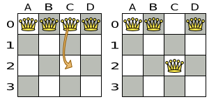
The new solution is called a neighbor of the original solution, because it can be
reached in a single Move. Although a single move can change multiple queens, the neighbors of a
solution should always be a very small subset of all possible solutions. For example, on that original solution,
these are all possible changeMove's:
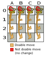
If we ignore the 4 changeMove's that have not impact and are therefore not doable, we can
see that number of moves is n * (n - 1) = 12. This is far less than the number of possible
solutions, which is n ^ n = 256. As the problem scales out, the number of possible moves
increases far less than the number of possible solutions.
Yet, in 4 changeMove's or less we can reach any solution. For example we can reach a very
different solution in 3 changeMove's:
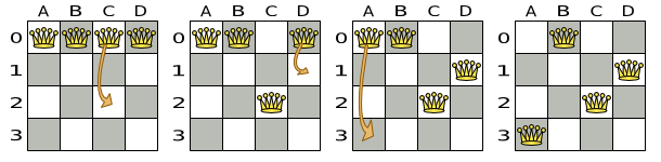
Note
There are many other types of moves besides changeMove's. Many move types are included
out-of-the-box, but you can also implement custom moves.
A Move can affect multiple entities or even create/delete entities. But it must not
change the problem facts.
All optimization algorithms use Move's to transition from one solution to a neighbor
solution. Therefore, all the optimization algorithms are confronted with Move selection: the
craft of creating and iterating moves efficiently and the art of finding the most promising subset of random moves
to evaluate first.
A MoveSelector's main function is to create Iterator<Move> when
needed. An optimization algorithm will iterate through a subset of those moves.
Here's an example how to configure a changeMoveSelector for the optimization algorithm
Local Search:
<localSearch>
<changeMoveSelector/>
...
</localSearch>Out of the box, this works and all properties of the changeMoveSelector are defaulted
sensibly (unless that fails fast due to ambiguity). On the other hand, the configuration can be customized
significantly for specific use cases. For example: you might want to configure a filter to discard pointless
moves.
To create a Move, a MoveSelector needs to select 1 or more planning
entities and/or planning values to move. Just like MoveSelectors,
EntitySelectors and ValueSelectors need to support a similar feature set
(such as scalable just-in-time selection). Therefore, they all implement a common interface
Selector and they are configured similarly.
A MoveSelector is often composed out of EntitySelectors,
ValueSelectors or even other MoveSelectors, which can be configured
individually if desired:
<unionMoveSelector>
<changeMoveSelector>
<entitySelector>
...
</entitySelector>
<valueSelector>
...
</valueSelector>
...
</changeMoveSelector>
<swapMoveSelector>
...
</swapMoveSelector>
</unionMoveSelector>Together, this structure forms a Selector tree:
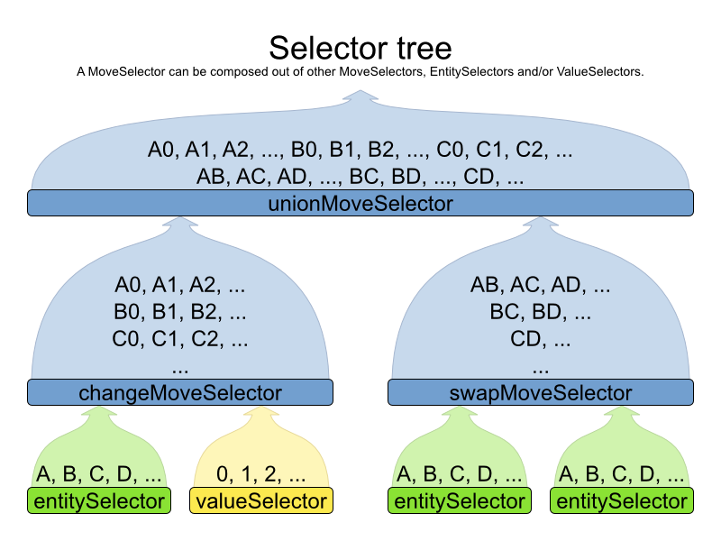
The root of this tree is a MoveSelector which is injected into the optimization algorithm
implementation to be (partially) iterated in every step.
For 1 planning variable, the ChangeMove selects 1 planning entity and 1 planning value
and assigns the entity's variable to that value.
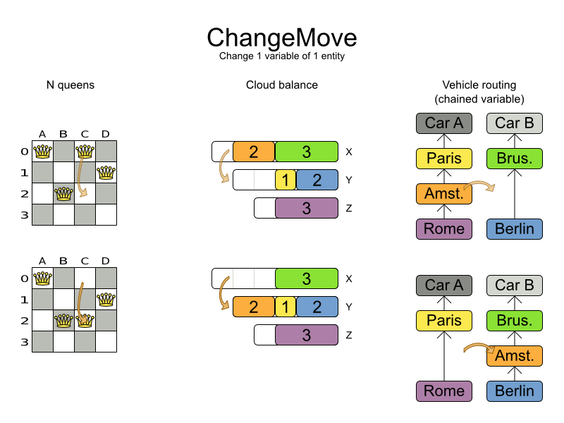
Simplest configuration:
<changeMoveSelector/>If there are multiple entity classes or multiple planning variables for 1 entity class, a simple
configuration will automatically unfold into a union of
ChangeMove selectors for every planning variable.
Advanced configuration:
<changeMoveSelector>
... <!-- Normal selector properties -->
<entitySelector>
<entityClass>...Lecture</entityClass>
...
</entitySelector>
<valueSelector>
<variableName>room</variableName>
...
<nearbySelection>...</nearbySelection>
</valueSelector>
</changeMoveSelector>A ChangeMove is the finest grained move.
Important
Almost every moveSelector configuration injected into a metaheuristic algorithm should
include a changeMoveSelector or a custom implementation. This guarantees that every possible
Solution can be reached through applying a number of moves in sequence (not taking score traps into account). Of course, normally it is unioned with other, more coarse
grained move selectors.
The SwapMove selects 2 different planning entities and swaps the planning values of all
their planning variables.
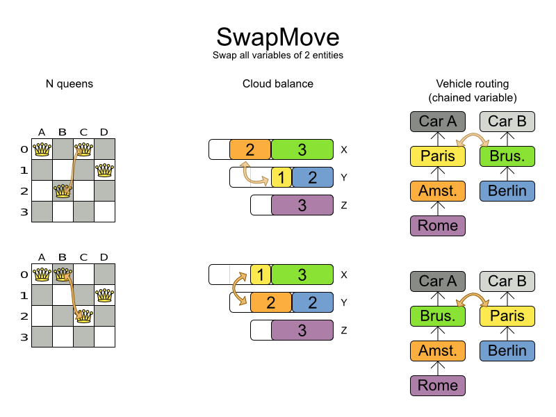
Although a SwapMove on a single variable is essentially just 2
ChangeMoves, it's often the winning step where the first of the 2
ChangeMoves would not be the winning step because it leaves the solution in a state with broken
hard constraints. For example: swapping the room of 2 lectures doesn't bring the solution in a intermediate state
where both lectures are in the same room which breaks a hard constraint.
Simplest configuration:
<swapMoveSelector/>If there are multiple entity classes, a simple configuration will automatically unfold into a union of SwapMove selectors for every entity class.
Advanced configuration:
<swapMoveSelector>
... <!-- Normal selector properties -->
<entitySelector>
<entityClass>...Lecture</entityClass>
...
</entitySelector>
<secondaryEntitySelector>
<entityClass>...Lecture</entityClass>
...
<nearbySelection>...</nearbySelection>
</secondaryEntitySelector>
<variableNameInclude>room</variableNameInclude>
<variableNameInclude>...</variableNameInclude>
</swapMoveSelector>The secondaryEntitySelector is rarely needed: if it is not specified, entities from the
same entitySelector are swapped.
If one or more variableNameInclude properties are specified, not all planning variables
will be swapped, but only those specified. For example for course scheduling, specifying only
variableNameInclude room will make it only swap room, not period.
A pillar is a set of planning entities which have the same planning value(s) for their
planning variable(s). The PillarChangeMove selects 1 entity pillar (or subset of those) and
changes the value of 1 variable (which is the same for all entities) to another value.
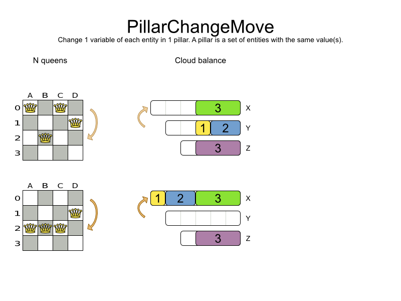
In the example above, queen A and C have the same value (row 0) and are moved to row 2. Also the yellow and blue process have the same value (computer Y) and are moved to computer X.
Simplest configuration:
<pillarChangeMoveSelector/>Advanced configuration:
<pillarSwapMoveSelector>
... <!-- Normal selector properties -->
<pillarSelector>
<entitySelector>
<entityClass>...Lecture</entityClass>
...
</entitySelector>
<subPillarEnabled>true</subPillarEnabled>
<minimumSubPillarSize>1</minimumSubPillarSize>
<maximumSubPillarSize>1000</maximumSubPillarSize>
</pillarSelector>
<valueSelector>
<variableName>room</variableName>
...
</valueSelector>
</pillarSwapMoveSelector>A sub pillar is a subset of entities that share the same value(s) for their variable(s). For example if
queen A, B, C and D are all located on row 0, they are a pillar and [A, D] is one of the many
sub pillars. If subPillarEnabled (defaults to true) is false, no sub pillars
are selected. If sub pillars are enabled, the pillar itself is also included and the properties
minimumSubPillarSize (defaults to 1) and
maximumSubPillarSize (defaults to infinity) limit the size of the selected
(sub) pillar.
Note
The number of sub pillars of a pillar is exponential to the size of the pillar. For example a pillar of
size 32 has (2^32 - 1) subpillars. Therefore a pillarSelector only
supports JIT random selection (which is the default).
The other properties are explained in changeMoveSelector.
A pillar is a set of planning entities which have the same planning value(s) for their
planning variable(s). The PillarSwapMove selects 2 different entity pillars and swaps the
values of all their variables for all their entities.
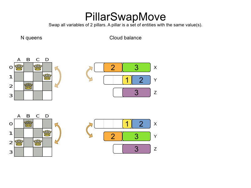
Simplest configuration:
<pillarSwapMoveSelector/>Advanced configuration:
<pillarSwapMoveSelector>
... <!-- Normal selector properties -->
<pillarSelector>
<entitySelector>
<entityClass>...Lecture</entityClass>
...
</entitySelector>
<subPillarEnabled>true</subPillarEnabled>
<minimumSubPillarSize>1</minimumSubPillarSize>
<maximumSubPillarSize>1000</maximumSubPillarSize>
</pillarSelector>
<secondaryPillarSelector>
<entitySelector>
...
</entitySelector>
...
</secondaryPillarSelector>
<variableNameInclude>room</variableNameInclude>
<variableNameInclude>...</variableNameInclude>
</pillarSwapMoveSelector>The secondaryPillarSelector is rarely needed: if it is not specified, entities from the
same pillarSelector are swapped.
The other properties are explained in swapMoveSelector and pillarChangeMoveSelector.
A tailChain is a set of planning entities with a chained planning variable which form a
last part of a chain. The tailChainSwapMove selects a tail chain and swaps it with the tail
chain of another planning value (in a different or the same anchor chain). If the targeted planning value, doesn't
have a tail chain, it swaps with nothing (resulting in a change like move). If it occurs within the same anchor
chain, a partial chain reverse occurs. In academic papers, this is often called a 2-opt move.
Simplest configuration:
<tailChainSwapMoveSelector/>Advanced configuration:
<subChainChangeMoveSelector>
... <!-- Normal selector properties -->
<entitySelector>
<entityClass>...Customer</entityClass>
...
</entitySelector>
<valueSelector>
<variableName>previousStandstill</variableName>
...
<nearbySelection>...</nearbySelection>
</valueSelector>
</subChainChangeMoveSelector>The entitySelector selects the start of the tail chain that is being moved. The
valueSelector selects to where that tail chain is moved. If it has a tail chain itself, that is moved to the
location of the original tail chain. It uses a valueSelector instead of a
secondaryEntitySelector to be able to include all possible 2opt moves (such as moving to the
end of a tail) and to work correctly with nearby selection (because of
asymmetric distances and also swapped entity distance gives an incorrect selection probability).
Note
Although subChainChangeMoveSelector and subChainSwapMoveSelector
include almost every possible tailChainSwapMove, experiments have shown that focusing on
tailChainSwapMoves increases efficiency.
A subChain is a set of planning entities with a chained planning variable which form
part of a chain. The subChainChangeMoveSelector selects a subChain and moves it to another
place (in a different or the same anchor chain).
Simplest configuration:
<subChainChangeMoveSelector/>Advanced configuration:
<subChainChangeMoveSelector>
... <!-- Normal selector properties -->
<entityClass>...Customer</entityClass>
<subChainSelector>
<valueSelector>
<variableName>previousStandstill</variableName>
...
</valueSelector>
<minimumSubChainSize>2</minimumSubChainSize>
<maximumSubChainSize>40</maximumSubChainSize>
</subChainSelector>
<valueSelector>
<variableName>previousStandstill</variableName>
...
</valueSelector>
<selectReversingMoveToo>true</selectReversingMoveToo>
</subChainChangeMoveSelector>The subChainSelector selects a number of entities, no less than
minimumSubChainSize (defaults to 1) and no more than
maximumSubChainSize (defaults to infinity).
Note
If minimumSubChainSize is 1 (which is the default), this selector
might select the same move as a ChangeMoveSelector, at a far lower selection probability
(because each move type has the same selection chance by default (not every move instance)
and there are far more SubChainChangeMove instances than ChangeMove
instances). However, don't just remove the ChangeMoveSelector, because experiments show that
it's good to focus on ChangeMoves.
Furthermore, in a SubChainSwapMoveSelector, setting
minimumSubChainSize prevents swapping a subchain of size 1 with a subchain
of at least size 2.
The selectReversingMoveToo property (defaults to true) enables selecting the reverse of
every subchain too.
The subChainSwapMoveSelector selects 2 different subChains and moves them to another
place in a different or the same anchor chain.
Simplest configuration:
<subChainSwapMoveSelector/>Advanced configuration:
<subChainSwapMoveSelector>
... <!-- Normal selector properties -->
<entityClass>...Customer</entityClass>
<subChainSelector>
<valueSelector>
<variableName>previousStandstill</variableName>
...
</valueSelector>
<minimumSubChainSize>2</minimumSubChainSize>
<maximumSubChainSize>40</maximumSubChainSize>
</subChainSelector>
<secondarySubChainSelector>
<valueSelector>
<variableName>previousStandstill</variableName>
...
</valueSelector>
<minimumSubChainSize>2</minimumSubChainSize>
<maximumSubChainSize>40</maximumSubChainSize>
</secondarySubChainSelector>
<selectReversingMoveToo>true</selectReversingMoveToo>
</subChainSwapMoveSelector>The secondarySubChainSelector is rarely needed: if it is not specified, entities from the
same subChainSelector are swapped.
The other properties are explained in subChainChangeMoveSelector.
A unionMoveSelector selects a Move by selecting 1 of its
MoveSelector children to supply the next Move.
Simplest configuration:
<unionMoveSelector>
<...MoveSelector/>
<...MoveSelector/>
<...MoveSelector/>
...
</unionMoveSelector>Advanced configuration:
<unionMoveSelector>
... <!-- Normal selector properties -->
<selectorProbabilityWeightFactoryClass>...ProbabilityWeightFactory</selectorProbabilityWeightFactoryClass>
<changeMoveSelector>
<fixedProbabilityWeight>...</fixedProbabilityWeight>
...
</changeMoveSelector>
<swapMoveSelector>
<fixedProbabilityWeight>...</fixedProbabilityWeight>
...
</swapMoveSelector>
<...MoveSelector>
<fixedProbabilityWeight>...</fixedProbabilityWeight>
...
</...MoveSelector>
...
</unionMoveSelector>The selectorProbabilityWeightFactory determines in selectionOrder
RANDOM how often a MoveSelector child is selected to supply the next Move.
By default, each MoveSelector child has the same chance of being selected.
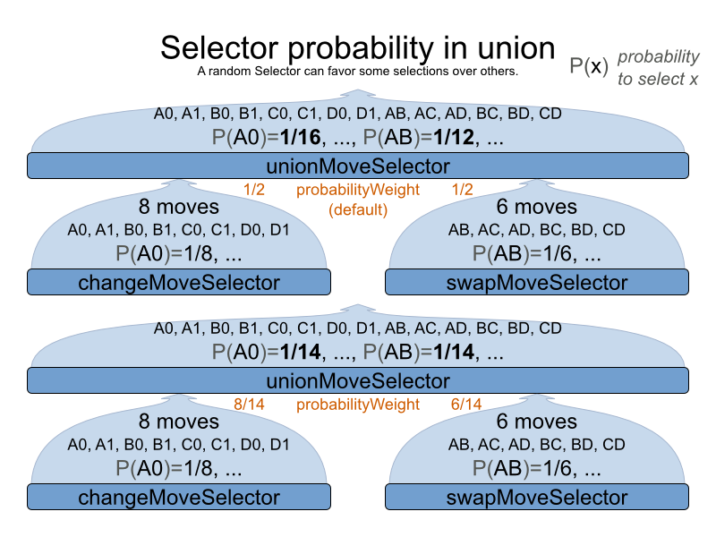
Change the fixedProbabilityWeight of such a child to select it more often. For example,
the unionMoveSelector can return a SwapMove twice as often as a
ChangeMove:
<unionMoveSelector>
<changeMoveSelector>
<fixedProbabilityWeight>1.0</fixedProbabilityWeight>
...
</changeMoveSelector>
<swapMoveSelector>
<fixedProbabilityWeight>2.0</fixedProbabilityWeight>
...
</swapMoveSelector>
</unionMoveSelector>The number of possible ChangeMoves is very different from the number of possible
SwapMoves and furthermore it's problem dependent. To give each individual
Move the same selection chance (as opposed to each MoveSelector), use the
FairSelectorProbabilityWeightFactory:
<unionMoveSelector>
<selectorProbabilityWeightFactoryClass>org.optaplanner.core.impl.heuristic.selector.common.decorator.FairSelectorProbabilityWeightFactory</selectorProbabilityWeightFactoryClass>
<changeMoveSelector/>
<swapMoveSelector/>
</unionMoveSelector>A cartesianProductMoveSelector selects a new CompositeMove. It builds
that CompositeMove by selecting 1 Move per MoveSelector
child and adding it to the CompositeMove.
Simplest configuration:
<cartesianProductMoveSelector>
<...MoveSelector/>
<...MoveSelector/>
<...MoveSelector/>
...
</cartesianProductMoveSelector>Advanced configuration:
<cartesianProductMoveSelector>
... <!-- Normal selector properties -->
<ignoreEmptyChildIterators>true</ignoreEmptyChildIterators>
<changeMoveSelector>
...
</changeMoveSelector>
<swapMoveSelector>
...
</swapMoveSelector>
<...MoveSelector>
...
</...MoveSelector>
...
</cartesianProductMoveSelector>The ignoreEmptyChildIterators property (true by default) will ignore every empty
childMoveSelector to avoid returning no moves. For example: a cartesian product of
changeMoveSelector A and B, for which B is empty (because all it's entities are immovable)
returns no move if ignoreEmptyChildIterators is false and the moves of A if
ignoreEmptyChildIterators is true.
Simplest configuration:
<entitySelector/>Advanced configuration:
<entitySelector>
... <!-- Normal selector properties -->
<entityClass>org.optaplanner.examples.curriculumcourse.domain.Lecture</entityClass>
</entitySelector>The entityClass property is only required if it cannot be deduced automatically because
there are multiple entity classes.
Simplest configuration:
<valueSelector/>Advanced configuration:
<valueSelector>
... <!-- Normal selector properties -->
<variableName>room</variableName>
</valueSelector>The variableName property is only required if it cannot be deduced automatically because
there are multiple variables (for the related entity class).
In exotic Construction Heuristic configurations, the entityClass from the
EntitySelector sometimes needs to be downcasted, which can be done with the property
downcastEntityClass:
<valueSelector>
<downcastEntityClass>...LeadingExam</downcastEntityClass>
<variableName>period</variableName>
</valueSelector>If a selected entity cannot be downcasted, the ValueSelector is empty for that
entity.
A Selector's cacheType determines when a selection (such as a
Move, an entity, a value, ...) is created and how long it lives.
Almost every Selector supports setting a cacheType:
<changeMoveSelector>
<cacheType>PHASE</cacheType>
...
</changeMoveSelector>The following cacheTypes are supported:
JUST_IN_TIME(default): Not cached. Construct each selection (Move, ...) just before it's used. This scales up well in memory footprint.STEP: Cached. Create each selection (Move, ...) at the beginning of a step and cache them in a list for the remainder of the step. This scales up badly in memory footprint.PHASE: Cached. Create each selection (Move, ...) at the beginning of a solver phase and cache them in a list for the remainder of the phase. Some selections cannot be phase cached because the list changes every step. This scales up badly in memory footprint, but has a slight performance gain.SOLVER: Cached. Create each selection (Move, ...) at the beginning of aSolverand cache them in a list for the remainder of theSolver. Some selections cannot be solver cached because the list changes every step. This scales up badly in memory footprint, but has a slight performance gain.
A cacheType can be set on composite selectors too:
<unionMoveSelector>
<cacheType>PHASE</cacheType>
<changeMoveSelector/>
<swapMoveSelector/>
...
</unionMoveSelector>Nested selectors of a cached selector cannot be configured to be cached themselves, unless it's a higher
cacheType. For example: a STEP cached unionMoveSelector
can hold a PHASE cached changeMoveSelector, but not a
STEP cached changeMoveSelector.
A Selector's selectionOrder determines the order in which the
selections (such as Moves, entities, values, ...) are iterated. An optimization algorithm will
usually only iterate through a subset of its MoveSelector's selections, starting from the
start, so the selectionOrder is critical to decide which Moves are actually
evaluated.
Almost every Selector supports setting a selectionOrder:
<changeMoveSelector>
...
<selectionOrder>RANDOM</selectionOrder>
...
</changeMoveSelector>The following selectionOrders are supported:
ORIGINAL: Select the selections (Moves, entities, values, ...) in default order. Each selection will be selected only once.For example: A0, A1, A2, A3, ..., B0, B1, B2, B3, ..., C0, C1, C2, C3, ...
SORTED: Select the selections (
Moves, entities, values, ...) in sorted order. Each selection will be selected only once. RequirescacheType >= STEP. Mostly used on anentitySelectororvalueSelectorfor construction heuristics. See sorted selection.For example: A0, B0, C0, ..., A2, B2, C2, ..., A1, B1, C1, ...
RANDOM (default): Select the selections (
Moves, entities, values, ...) in non-shuffled random order. A selection might be selected multiple times. This scales up well in performance because it does not require caching.For example: C2, A3, B1, C2, A0, C0, ...
SHUFFLED: Select the selections (
Moves, entities, values, ...) in shuffled random order. Each selection will be selected only once. RequirescacheType >= STEP. This scales up badly in performance, not just because it requires caching, but also because a random number is generated for each element, even if it's not selected (which is the grand majority when scaling up).For example: C2, A3, B1, A0, C0, ...
PROBABILISTIC: Select the selections (
Moves, entities, values, ...) in random order, based on the selection probability of each element. A selection with a higher probability has a higher chance to be selected than elements with a lower probability. A selection might be selected multiple times. RequirescacheType >= STEP. Mostly used on anentitySelectororvalueSelector. See probabilistic selection.For example: B1, B1, A1, B2, B1, C2, B1, B1, ...
A selectionOrder can be set on composite selectors too.
Note
When a Selector is cached, all of its nested Selectors will
naturally default to selectionOrder ORIGINAL. Avoid overwriting the
selectionOrder of those nested Selectors.
This combination is great for big use cases (10 000 entities or more), as it scales up well in memory
footprint and performance. Other combinations are often not even viable on such sizes. It works for smaller use
cases too, so it's a good way to start out. It's the default, so this explicit configuration of
cacheType and selectionOrder is actually obsolete:
<unionMoveSelector>
<cacheType>JUST_IN_TIME</cacheType>
<selectionOrder>RANDOM</selectionOrder>
<changeMoveSelector/>
<swapMoveSelector/>
</unionMoveSelector>Here's how it works. When Iterator<Move>.next() is called, a child
MoveSelector is randomly selected (1), which creates a random Move (2, 3,
4) and is then returned (5):
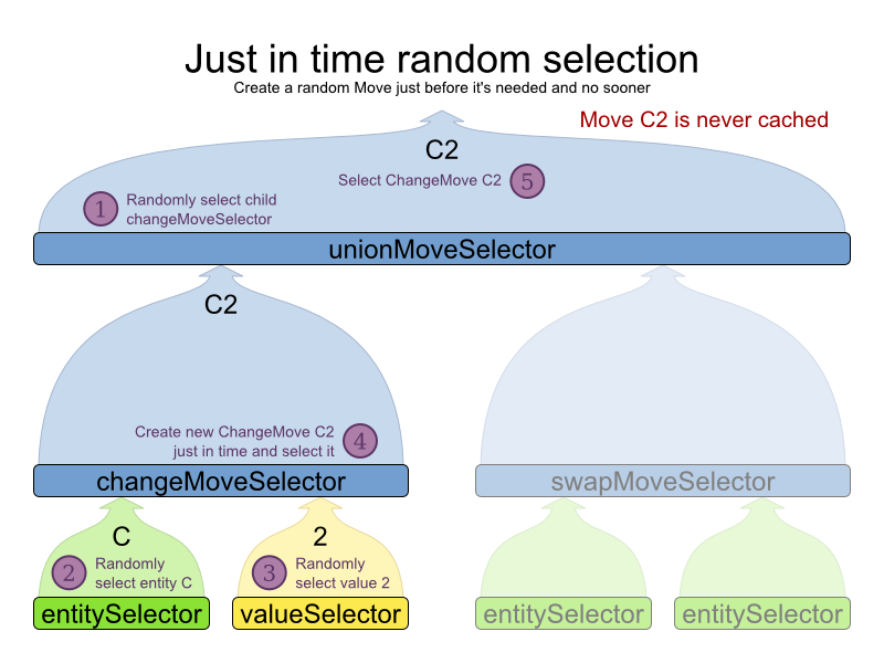
Notice that it never creates a list of Moves and it
generates random numbers only for Moves that are actually selected.
This combination often wins for small and medium use cases (5000 entities or less). Beyond that size, it scales up badly in memory footprint and performance.
<unionMoveSelector>
<cacheType>PHASE</cacheType>
<selectionOrder>SHUFFLED</selectionOrder>
<changeMoveSelector/>
<swapMoveSelector/>
</unionMoveSelector>Here's how it works: At the start of the phase (or step depending on the cacheType),
all moves are created (1) and cached (2). When MoveSelector.iterator() is called, the moves
are shuffled (3). When Iterator<Move>.next() is called, the next element in the
shuffled list is returned (4):
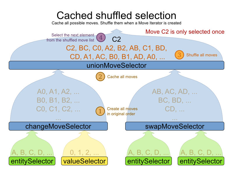
Notice that each Move will only be selected once, even
though they are selected in random order.
Use cacheType PHASE if none of the (possibly nested) Selectors require STEP. Otherwise,
do something like this:
<unionMoveSelector>
<cacheType>STEP</cacheType>
<selectionOrder>SHUFFLED</selectionOrder>
<changeMoveSelector>
<cacheType>PHASE</cacheType>
</changeMoveSelector>
<swapMoveSelector/>
<cacheType>PHASE</cacheType>
</swapMoveSelector>
<pillarSwapMoveSelector/><!-- Does not support cacheType PHASE -->
</unionMoveSelector>This combination is often a worthy competitor for medium use cases, especially with fast stepping optimization algorithms (such as Simulated Annealing). Unlike cached shuffled selection, it doesn't waste time shuffling the moves list at the beginning of every step.
<unionMoveSelector>
<cacheType>PHASE</cacheType>
<selectionOrder>RANDOM</selectionOrder>
<changeMoveSelector/>
<swapMoveSelector/>
</unionMoveSelector>There can be certain moves that you don't want to select, because:
The move is pointless and would only waste CPU time. For example, swapping 2 lectures of the same course will result in the same score and the same schedule because all lectures of 1 course are interchangeable (same teacher, same students, same topic).
Doing the move would break a built-in hard constraint, so the solution would be infeasible but the score function doesn't check built-in hard constraints (for performance gain). For example, don't change a gym lecture to a room which is not a gym room.
Note
Any built-in hard constraint must probably be filtered on every move type of every solver phase. For example if it's filters the change move of Local Search, it must also filter the swap move that swaps the room of a gym lecture with another lecture for which the other lecture's original room isn't a gym room. Furthermore, it must also filter the change moves of the Construction Heuristics (which requires an advanced configuration).
Filtered selection can happen on any Selector in the selector tree, including any
MoveSelector, EntitySelector or ValueSelector. It works
with any cacheType and selectionOrder.
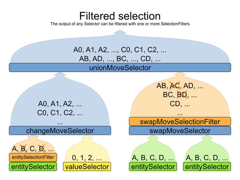
Filtering uses the interface SelectionFilter:
public interface SelectionFilter<T> {
boolean accept(ScoreDirector scoreDirector, T selection);
}Implement the accept method to return false on a discarded
selection. Unaccepted moves will not be selected and will therefore never have their
doMove method called.
public class DifferentCourseSwapMoveFilter implements SelectionFilter<SwapMove> {
public boolean accept(ScoreDirector scoreDirector, SwapMove move) {
Lecture leftLecture = (Lecture) move.getLeftEntity();
Lecture rightLecture = (Lecture) move.getRightEntity();
return !leftLecture.getCourse().equals(rightLecture.getCourse());
}
}Apply the filter on the lowest level possible. In most cases, you'll need to know both the entity and the
value involved and you'll have to apply a filterClass on the
moveSelector:
<swapMoveSelector>
<filterClass>org.optaplanner.examples.curriculumcourse.solver.move.DifferentCourseSwapMoveFilter</filterClass>
</swapMoveSelector>But if possible, apply it on a lower levels, such as a filterClass on the
entitySelector or valueSelector:
<changeMoveSelector>
<entitySelector>
<filterClass>...EntityFilter</filterClass>
</entitySelector>
</changeMoveSelector>You can configure multiple filterClass elements on a single selector.
Sorted selection can happen on any Selector in the selector tree, including any
MoveSelector, EntitySelector or ValueSelector. It does
not work with cacheType JUST_IN_TIME and it only works with
selectionOrder SORTED.
It's mostly used in construction heuristics.
Note
If the chosen construction heuristic implies sorting, for example FIRST_FIT_DECREASING
implies that the EntitySelector is sorted, there is no need to explicitly configure a
Selector with sorting. If you do explicitly configure the Selector, it
overwrites the default settings of that construction heuristic.
Some Selector types implement a SorterManner out of the box:
EntitySelectorsupports:DECREASING_DIFFICULTY: Sorts the planning entities according to decreasing planning entity difficulty. Requires that planning entity difficulty is annotated on the domain model.<entitySelector> <cacheType>PHASE</cacheType> <selectionOrder>SORTED</selectionOrder> <sorterManner>DECREASING_DIFFICULTY</sorterManner> </entitySelector>
ValueSelectorsupports:INCREASING_STRENGTH: Sorts the planning values according to increasing planning value strength. Requires that planning value strength is annotated on the domain model.<valueSelector> <cacheType>PHASE</cacheType> <selectionOrder>SORTED</selectionOrder> <sorterManner>INCREASING_STRENGTH</sorterManner> </valueSelector>
An easy way to sort a Selector is with a plain old
Comparator:
public class CloudProcessDifficultyComparator implements Comparator<CloudProcess> {

    public int compare(CloudProcess a, CloudProcess b) {
        return new CompareToBuilder()
                .append(a.getRequiredMultiplicand(), b.getRequiredMultiplicand())
                .append(a.getId(), b.getId())
                .toComparison();
    }

}You 'll also need to configure it (unless it's annotated on the domain model and automatically applied by the optimization algorithm):
<entitySelector>
<cacheType>PHASE</cacheType>
<selectionOrder>SORTED</selectionOrder>
<sorterComparatorClass>...CloudProcessDifficultyComparator</sorterComparatorClass>
<sorterOrder>DESCENDING</sorterOrder>
</entitySelector>If you need the entire Solution to sort a Selector, use a
SelectionSorterWeightFactory instead:
public interface SelectionSorterWeightFactory<Sol extends Solution, T> {
Comparable createSorterWeight(Sol solution, T selection);
}public class QueenDifficultyWeightFactory implements SelectionSorterWeightFactory<NQueens, Queen> {
public Comparable createSorterWeight(NQueens nQueens, Queen queen) {
int distanceFromMiddle = calculateDistanceFromMiddle(nQueens.getN(), queen.getColumnIndex());
return new QueenDifficultyWeight(queen, distanceFromMiddle);
}
// ...
public static class QueenDifficultyWeight implements Comparable<QueenDifficultyWeight> {
private final Queen queen;
private final int distanceFromMiddle;
public QueenDifficultyWeight(Queen queen, int distanceFromMiddle) {
this.queen = queen;
this.distanceFromMiddle = distanceFromMiddle;
}
public int compareTo(QueenDifficultyWeight other) {
return new CompareToBuilder()
// The more difficult queens have a lower distance to the middle
.append(other.distanceFromMiddle, distanceFromMiddle) // Decreasing
// Tie breaker
.append(queen.getColumnIndex(), other.queen.getColumnIndex())
.toComparison();
}
}
}You 'll also need to configure it (unless it's annotated on the domain model and automatically applied by the optimization algorithm):
<entitySelector>
<cacheType>PHASE</cacheType>
<selectionOrder>SORTED</selectionOrder>
<sorterWeightFactoryClass>...QueenDifficultyWeightFactory</sorterWeightFactoryClass>
<sorterOrder>DESCENDING</sorterOrder>
</entitySelector>Alternatively, you can also use the interface SelectionSorter directly:
public interface SelectionSorter<T> {
void sort(ScoreDirector scoreDirector, List<T> selectionList);
} <entitySelector>
<cacheType>PHASE</cacheType>
<selectionOrder>SORTED</selectionOrder>
<sorterClass>...MyEntitySorter</sorterClass>
</entitySelector>Probabilistic selection can happen on any Selector in the selector tree, including any
MoveSelector, EntitySelector or ValueSelector. It does
not work with cacheType JUST_IN_TIME and it only works with
selectionOrder PROBABILISTIC.
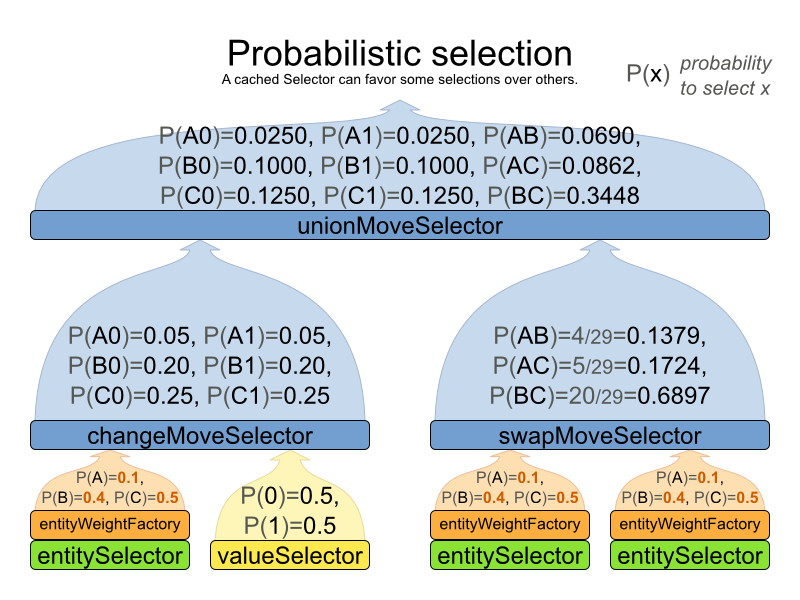
Each selection has a probabilityWeight, which determines the chance that selection will
be selected:
public interface SelectionProbabilityWeightFactory<T> {
double createProbabilityWeight(ScoreDirector scoreDirector, T selection);
} <entitySelector>
<cacheType>PHASE</cacheType>
<selectionOrder>PROBABILISTIC</selectionOrder>
<probabilityWeightFactoryClass>...MyEntityProbabilityWeightFactoryClass</probabilityWeightFactoryClass>
</entitySelector>For example, if there are 3 entities: process A (probabilityWeight 2.0), process B (probabilityWeight 0.5) and process C (probabilityWeight 0.5), then process A will be selected 4 times more than B and C.
Selecting all possible moves sometimes does not scale well enough, especially for construction heuristics (which don't support acceptedCountLimit).
To limit the number of selected selection per step, apply a selectedCountLimit on the
selector:
<changeMoveSelector>
<selectedCountLimit>100</selectedCountLimit>
</changeMoveSelector>Note
To scale Local Search, setting acceptedCountLimit is usually
better than using selectedCountLimit.
During mimic selection, 1 normal selector records its selection and 1 or multiple other special selectors replay that selection. The recording selector acts as a normal selector and supports all other configuration properties. A replaying selector mimics the recording selection and support no other configuration properties.
The recording selector needs an id. A replaying selector must reference a recorder's id
with a mimicSelectorRef:
<cartesianProductMoveSelector>
<changeMoveSelector>
<entitySelector id="entitySelector"/>
<valueSelector>
<variableName>period</variableName>
</valueSelector>
</changeMoveSelector>
<changeMoveSelector>
<entitySelector mimicSelectorRef="entitySelector"/>
<valueSelector>
<variableName>room</variableName>
</valueSelector>
</changeMoveSelector>
</cartesianProductMoveSelector>Mimic selection is useful to create a composite move from 2 moves that affect the same entity.
In some use cases (such as TSP and VRP, but also in non-chained variable cases), changing entities to nearby values or swapping nearby entities can heavily increase scalability and improve solution quality.
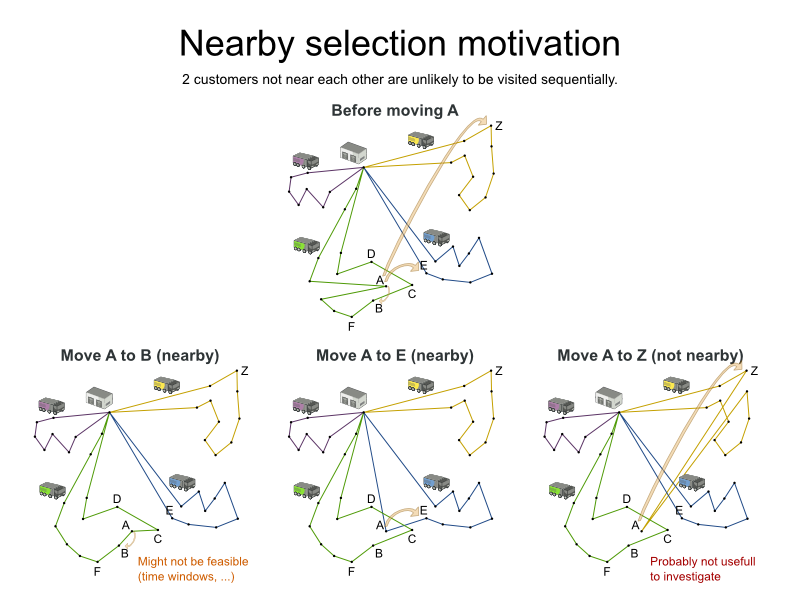
Nearby selection increases the probability of selecting an entity or value which is nearby to the first entity being moved in that move.
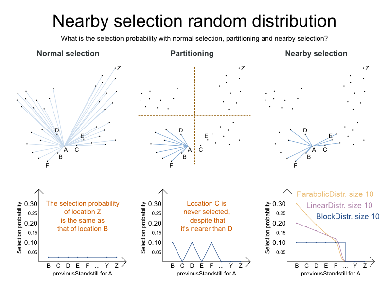
The distance between 2 entities or values is domain specific. Therefore, implement the
NearbyDistanceMeter interface:
public interface NearbyDistanceMeter<O, D> {
double getNearbyDistance(O origin, D destination);
}It returns a double which represents the distance:
public class CustomerNearbyDistanceMeter implements NearbyDistanceMeter<Customer, Standstill> {
public double getNearbyDistance(Customer origin, Standstill destination) {
return origin.getDistanceTo(destination);
}
}To configure nearby selection, add a nearbySelection element in the
entitySelector or valueSelector and use mimic
selection to specify which entity should be near by the selection.
<unionMoveSelector>
<changeMoveSelector>
<entitySelector id="entitySelector1"/>
<valueSelector>
<nearbySelection>
<originEntitySelector mimicSelectorRef="entitySelector1"/>
<nearbyDistanceMeterClass>...CustomerNearbyDistanceMeter</nearbyDistanceMeterClass>
<parabolicDistributionSizeMaximum>40</parabolicDistributionSizeMaximum>
</nearbySelection>
</valueSelector>
</changeMoveSelector>
<swapMoveSelector>
<entitySelector id="entitySelector2"/>
<secondaryEntitySelector>
<nearbySelection>
<originEntitySelector mimicSelectorRef="entitySelector2"/>
<nearbyDistanceMeterClass>...CustomerNearbyDistanceMeter</nearbyDistanceMeterClass>
<parabolicDistributionSizeMaximum>40</parabolicDistributionSizeMaximum>
</nearbySelection>
</secondaryEntitySelector>
</swapMoveSelector>
<tailChainSwapMoveSelector>
<entitySelector id="entitySelector3"/>
<valueSelector>
<nearbySelection>
<originEntitySelector mimicSelectorRef="entitySelector3"/>
<nearbyDistanceMeterClass>...CustomerNearbyDistanceMeter</nearbyDistanceMeterClass>
<parabolicDistributionSizeMaximum>40</parabolicDistributionSizeMaximum>
</nearbySelection>
</valueSelector>
</tailChainSwapMoveSelector>
</unionMoveSelector>To allow every element to be selected, regardless of the number of entities, only set the distribution type without the size maximum parameter:
<nearbySelection>
<nearbySelectionDistributionType>PARABOLIC_DISTRIBUTION</nearbySelectionDistributionType>
</nearbySelection>The following NearbySelectionDistributionTypes are supported:
BLOCK_DISTRIBUTION: Only the n nearest are selected, with an equal probability. For example, select the 20 nearest:<nearbySelection> <blockDistributionSizeMaximum>20</blockDistributionSizeMaximum> </nearbySelection>LINEAR_DISTRIBUTION: Nearest elements are selected with a higher probability. The probability decreases linearly.<nearbySelection> <linearDistributionSizeMaximum>40</linearDistributionSizeMaximum> </nearbySelection>PARABOLIC_DISTRIBUTION(recommended): Nearest elements are selected with a higher probability.<nearbySelection> <parabolicDistributionSizeMaximum>80</parabolicDistributionSizeMaximum> </nearbySelection>BETA_DISTRIBUTION: Selection according to a beta distribution. Slows down the solver significantly.<nearbySelection> <betaDistributionAlpha>1</betaDistributionAlpha> <betaDistributionBeta>5</betaDistributionBeta> </nearbySelection>
As always, use the Benchmarker to tweak values if desired.
To determine which move types might be missing in your implementation, run a Benchmarker for a short amount of time and configure it to write the best solutions to disk. Take a look at such a best solution: it will likely be a local optima. Try to figure out if there's a move that could get out of that local optima faster.
If you find one, implement that coarse-grained move, mix it with the existing moves and benchmark it against the previous configurations to see if you want to keep it.
Instead of reusing the generic Moves (such as ChangeMove) you can also
implement your own Moves. Generic and custom MoveSelectors can be combined
as desired.
A custom Move can be tailored to work to the advantage of your constraints. For example,
in examination scheduling, changing the period of an exam A also changes the period of all the exams that need to
coincide with exam A.
A custom Move is also slightly faster than a generic Move. However,
it's far more work to implement and much harder to avoid bugs. After implementing a custom
Move, make sure to turn on environmentMode FULL_ASSERT to
check for score corruptions.
Your custom moves must implement the Move interface:
public interface Move {
boolean isMoveDoable(ScoreDirector scoreDirector);
Move createUndoMove(ScoreDirector scoreDirector);
void doMove(ScoreDirector scoreDirector);
Collection<? extends Object> getPlanningEntities();
Collection<? extends Object> getPlanningValues();
}Let's take a look at the Move implementation for 4 queens which moves a queen to a
different row:
public class RowChangeMove extends AbstractMove {
private Queen queen;
private Row toRow;
public RowChangeMove(Queen queen, Row toRow) {
this.queen = queen;
this.toRow = toRow;
}
// ... see below
}An instance of RowChangeMove moves a queen from its current row to a different
row.
Planner calls the doMove(ScoreDirector) method to do a move. The Move
implementation must notify the ScoreDirector of any changes it makes to planning entity's
variables:
public void doMove(ScoreDirector scoreDirector) {
scoreDirector.beforeVariableChanged(queen, "row"); // before changes are made to the queen.row
queen.setRow(toRow);
scoreDirector.afterVariableChanged(queen, "row"); // after changes are made to the queen.row
}You need to call the scoreDirector.beforeVariableChanged(Object, String) and
scoreDirector.afterVariableChanged(Object, String) methods directly before and after modifying
the entity.
Note
You can alter multiple entities in a single move and effectively create a big move (also known as a coarse-grained move).
Warning
A Move can only change/add/remove planning entities, it must not change any of the
problem facts.
Planner automatically filters out non doable moves by calling the
isMoveDoable(ScoreDirector) method on a move. A non doable move is:
A move that changes nothing on the current solution. For example, moving queen B0 to row 0 is not doable, because it is already there.
A move that is impossible to do on the current solution. For example, moving queen B0 to row 10 is not doable because it would move it outside the board limits.
In the n queens example, a move which moves the queen from its current row to the same row isn't doable:
public boolean isMoveDoable(ScoreDirector scoreDirector) {
return !ObjectUtils.equals(queen.getRow(), toRow);
}Because we won't generate a move which can move a queen outside the board limits, we don't need to check it.
A move that is currently not doable could become doable on the working Solution of a later
step.
Each move has an undo move: a move (normally of the same type) which does the exact
opposite. In the example above the undo move of C0 to C2 would be the move C2 to
C0. An undo move is created from a Move, before the Move has been
done on the current solution.
public Move createUndoMove(ScoreDirector scoreDirector) {
return new RowChangeMove(queen, queen.getRow());
}Notice that if C0 would have already been moved to C2, the undo move would create the move C2 to C2, instead of the move C2 to C0.
A solver phase might do and undo the same Move more than once. In fact, many solver
phases will iteratively do and undo a number of moves to evaluate them, before selecting one of those and doing
that move again (without undoing it this time).
A Move must implement the getPlanningEntities() and
getPlanningValues() methods. They are used by entity tabu and value tabu respectively. When
they are called, the Move has already been done.
public List<? extends Object> getPlanningEntities() {
return Collections.singletonList(queen);
}
public Collection<? extends Object> getPlanningValues() {
return Collections.singletonList(toRow);
}If your Move changes multiple planning entities, return all of them in
getPlanningEntities() and return all their values (to which they are changing) in
getPlanningValues().
public Collection<? extends Object> getPlanningEntities() {
return Arrays.asList(leftCloudProcess, rightCloudProcess);
}
public Collection<? extends Object> getPlanningValues() {
return Arrays.asList(leftCloudProcess.getComputer(), rightCloudProcess.getComputer());
}A Move must implement the equals() and hashCode()
methods. 2 moves which make the same change on a solution, should be equal.
public boolean equals(Object o) {
if (this == o) {
return true;
} else if (o instanceof RowChangeMove) {
RowChangeMove other = (RowChangeMove) o;
return new EqualsBuilder()
.append(queen, other.queen)
.append(toRow, other.toRow)
.isEquals();
} else {
return false;
}
}
public int hashCode() {
return new HashCodeBuilder()
.append(queen)
.append(toRow)
.toHashCode();
}Notice that it checks if the other move is an instance of the same move type. This
instanceof check is important because a move will be compared to a move with another move type
if you're using more than 1 move type.
Implement the toString() method to keep Planner's logs readable:
public String toString() {
return queen + " {" + queen.getRow() + " -> " + toRow + "}";
}Now that we can implement a single custom Move, let's take a look at generating such
custom moves.
The easiest way to generate custom moves is by implementing the interface
MoveListFactory:
public interface MoveListFactory<S extends Solution> {
List<Move> createMoveList(S solution);
}For example:
public class RowChangeMoveFactory implements MoveListFactory<NQueens> {
public List<Move> createMoveList(NQueens nQueens) {
List<Move> moveList = new ArrayList<Move>();
for (Queen queen : nQueens.getQueenList()) {
for (Row toRow : nQueens.getRowList()) {
moveList.add(new RowChangeMove(queen, toRow));
}
}
return moveList;
}
}Simple configuration (which can be nested in a unionMoveSelector just like any other
MoveSelector):
<moveListFactory>
<moveListFactoryClass>org.optaplanner.examples.nqueens.solver.move.factory.RowChangeMoveFactory</moveListFactoryClass>
</moveListFactory>Advanced configuration:
<moveListFactory>
... <!-- Normal moveSelector properties -->
<moveListFactoryClass>org.optaplanner.examples.nqueens.solver.move.factory.RowChangeMoveFactory</moveListFactoryClass>
</moveListFactory>Because the MoveListFactory generates all moves at once in a
List<Move>, it does not support cacheType
JUST_IN_TIME. Therefore, moveListFactory uses cacheType
STEP by default and it scales badly in memory footprint.
Use this advanced form to generate custom moves by implementing the MoveIteratorFactory
interface:
public interface MoveIteratorFactory {
long getSize(ScoreDirector scoreDirector);
Iterator<Move> createOriginalMoveIterator(ScoreDirector scoreDirector);
Iterator<Move> createRandomMoveIterator(ScoreDirector scoreDirector, Random workingRandom);
}The getSize() method must give an estimation of the size. It doesn't need to be correct.
The createOriginalMoveIterator method is called if the selectionOrder is
ORIGINAL or if it is cached. The createRandomMoveIterator method is called
for selectionOrder RANDOM combined with cacheType
JUST_IN_TIME.
Important
Don't create a collection (list, array, map, set) of Moves when creating the
Iterator<Move>: the whole purpose of MoveIteratorFactory over
MoveListFactory is giving you the ability to create a Move just in time in
the Iterator's method next().
Simple configuration (which can be nested in a unionMoveSelector just like any other
MoveSelector):
<moveIteratorFactory>
<moveIteratorFactoryClass>...</moveIteratorFactoryClass>
</moveIteratorFactory>Advanced configuration:
<moveIteratorFactory>
... <!-- Normal moveSelector properties -->
<moveIteratorFactoryClass>...</moveIteratorFactoryClass>
</moveIteratorFactory>Exhaustive Search will always find the global optimum and recognize it too. That being said, it doesn't scale (not even beyond toy data sets) and is therefore mostly useless.
The Brute Force algorithm creates and evaluates every possible solution.
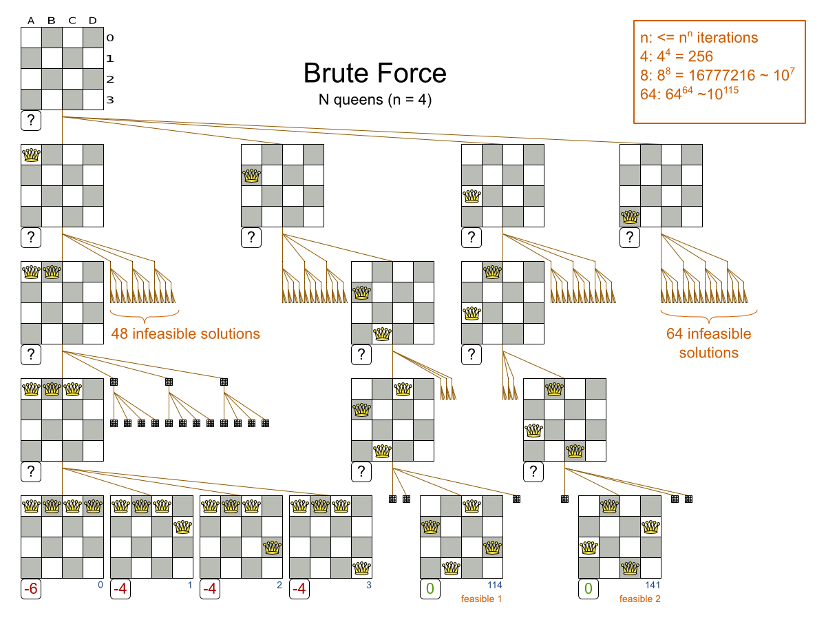
Notice that it creates a search tree that explodes exponentially as the problem size increases, so it hits a scalability wall.
Important
Brute Force is mostly unusable for a real-world problem due to time limitations, as shown in scalability of Exhaustive Search.
Branch And Bound also explores nodes in an exponential search tree, but it investigates more promising nodes first and prunes away worthless nodes.
For each node, Branch And Bound calculates the optimistic bound: the best possible score to which that node can lead to. If the optimistic bound of a node is lower or equal to the global pessimistic bound, then it prunes away that node (including the entire branch of all its subnodes).
Note
Academic papers use the term lower bound instead of optimistic bound (and the term upper bound instead of pessimistic bound), because they minimize the score.
Planner maximizes the score (because it supports combining negative and positive constraints). Therefore, for clarity, it uses different terms, as it would be confusing to use the term lower bound for a bound which is always higher.
For example: at index 15, it can prune away all unvisited solutions with queen A on row 0, because none will
be better than the solution of index 14 with a score of -1.
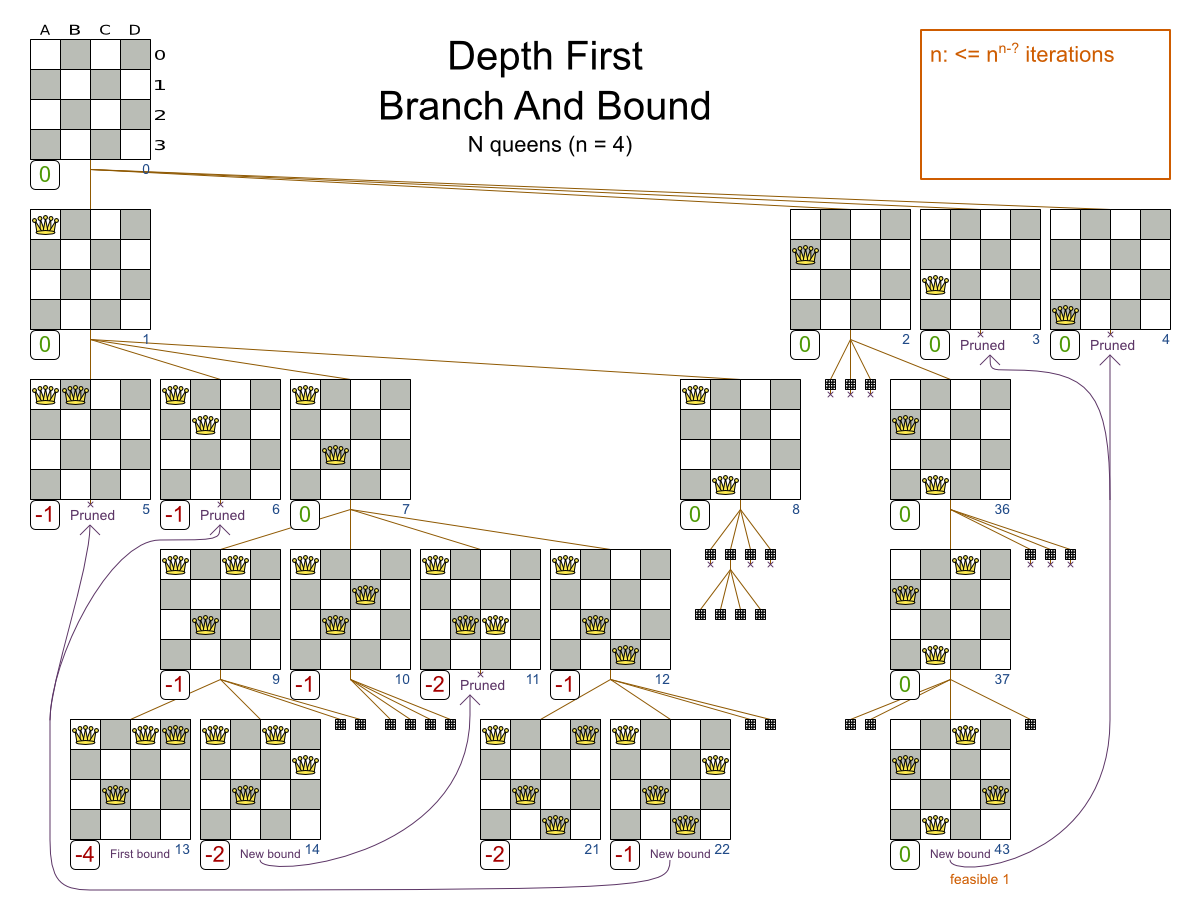
Notice that Branch And Bound (much like Brute Force) creates a search tree that explodes exponentially as the problem size increases. So it hits the same scalability wall, only a little bit later.
Important
Branch And Bound is mostly unusable for a real-world problem due to time limitations, as shown in scalability of Exhaustive Search.
Simplest configuration of Branch And Bound:
<solver>
...
<exhaustiveSearch>
<exhaustiveSearchType>BRANCH_AND_BOUND</exhaustiveSearchType>
</exhaustiveSearch>
</solver>Important
For the pruning to work with the default ScoreBounder, the InitializingScoreTrend should be set. Especially an InitializingScoreTrend of ONLY_DOWN (or at least has
ONLY_DOWN in the leading score levels) prunes a lot.
Advanced configuration:
<exhaustiveSearch>
<exhaustiveSearchType>BRANCH_AND_BOUND</exhaustiveSearchType>
<nodeExplorationType>DEPTH_FIRST</nodeExplorationType>
<entitySorterManner>DECREASING_DIFFICULTY_IF_AVAILABLE</entitySorterManner>
<valueSorterManner>INCREASING_STRENGTH_IF_AVAILABLE</valueSorterManner>
</exhaustiveSearch>The nodeExplorationType options are:
DEPTH_FIRST(default): Explore deeper nodes first (and then a better score and then a better optimistic bound). Deeper nodes (especially leaf nodes) often improve the pessimistic bound. A better pessimistic bound allows pruning more nodes to reduce the search space.<exhaustiveSearch> <exhaustiveSearchType>BRANCH_AND_BOUND</exhaustiveSearchType> <nodeExplorationType>DEPTH_FIRST</nodeExplorationType> </exhaustiveSearch>BREADTH_FIRST(not recommended): Explore nodes layer by layer (and then a better score and then a better optimistic bound). Scales terribly in memory (and usually in performance too).<exhaustiveSearch> <exhaustiveSearchType>BRANCH_AND_BOUND</exhaustiveSearchType> <nodeExplorationType>BREADTH_FIRST</nodeExplorationType> </exhaustiveSearch>SCORE_FIRST: Explore nodes with a better score first (and then a better optimistic bound and then deeper nodes first). Might scale as terribly asBREADTH_FIRSTin some cases.<exhaustiveSearch> <exhaustiveSearchType>BRANCH_AND_BOUND</exhaustiveSearchType> <nodeExplorationType>SCORE_FIRST</nodeExplorationType> </exhaustiveSearch>OPTIMISTIC_BOUND_FIRST: Explore nodes with a better optimistic bound first (and then a better score and then deeper nodes first). Might scale as terribly asBREADTH_FIRSTin some cases.<exhaustiveSearch> <exhaustiveSearchType>BRANCH_AND_BOUND</exhaustiveSearchType> <nodeExplorationType>OPTIMISTIC_BOUND_FIRST</nodeExplorationType> </exhaustiveSearch>
The entitySorterManner options are:
DECREASING_DIFFICULTY: Initialize the more difficult planning entities first. This usually increases pruning (and therefore improves scalability). Requires the model to support planning entity difficulty comparison.DECREASING_DIFFICULTY_IF_AVAILABLE(default): If the model supports planning entity difficulty comparison, behave likeDECREASING_DIFFICULTY, else likeNONE.NONE: Initialize the planning entities in original order.
The valueSorterManner options are:
INCREASING_STRENGTH: Evaluate the planning values in increasing strength. Requires the model to support planning value strength comparison.INCREASING_STRENGTH_IF_AVAILABLE(default): If the model supports planning value strength comparison, behave likeINCREASING_STRENGTH, else likeNONE.DECREASING_STRENGTH: Evaluate the planning values in decreasing strength. Requires the model to support planning value strength comparison.DECREASING_STRENGTH_IF_AVAILABLE: If the model supports planning value strength comparison, behave likeDECREASING_STRENGTH, else likeNONE.NONE: Try the planning values in original order.
Exhaustive Search variants suffer from 2 big scalability issues:
They scale terribly memory wise.
They scale horribly performance wise.
As shown in these time spent graphs from the Benchmarker, Brute Force and Branch And Bound both hit a performance scalability wall. For example, on N queens it hits wall at a few dozen queens:
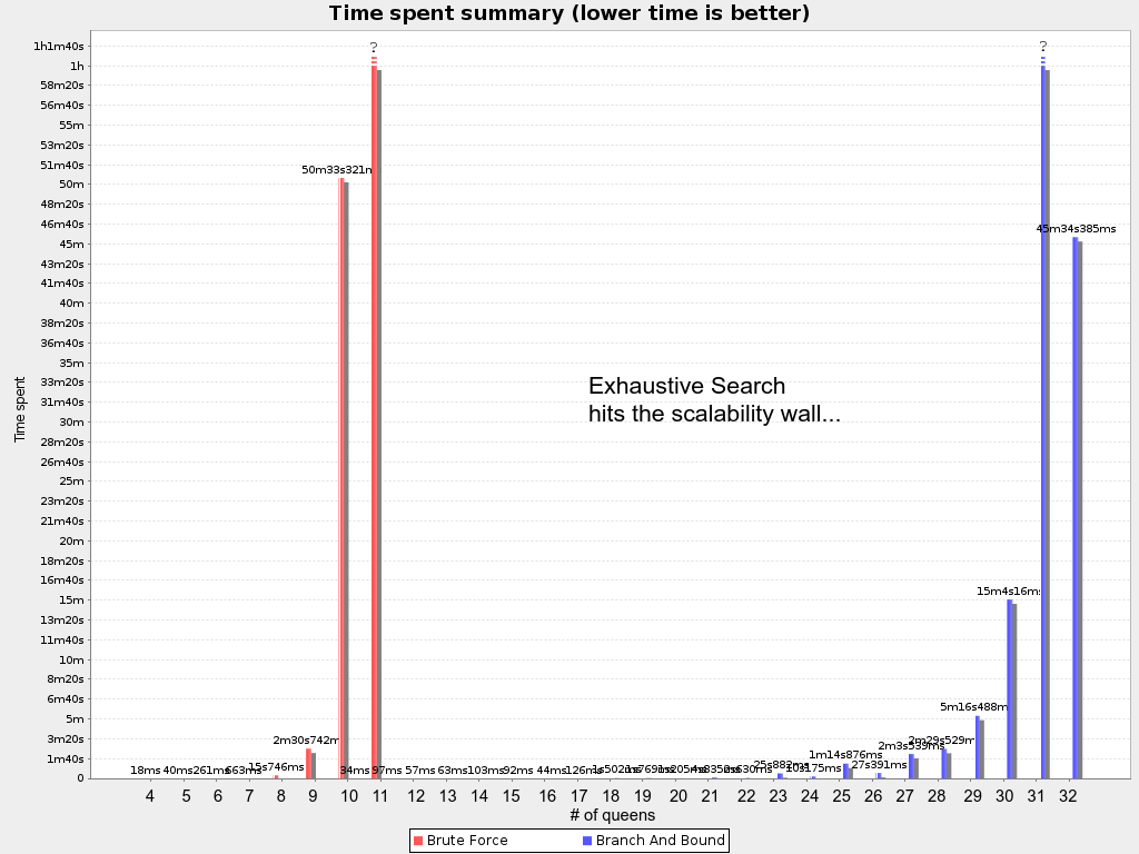
In most use cases, such as Cloud Balancing, the wall appears out of thin air:
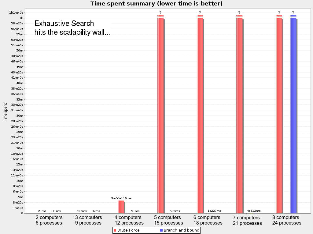
Exhaustive Search hits this wall on small datasets already, so in production these optimizations algorithms are mostly useless. Use Construction Heuristics with Local Search instead: those can handle thousands of queens/computers easily.
Note
Throwing hardware at these scalability issues has no noticeable impact. Newer and more hardware are just a drop in the ocean. Moore's law cannot win against the onslaught of a few more planning entities in the dataset.
A construction heuristic builds a pretty good initial solution in a finite length of time. Its solution isn't always feasible, but it finds it fast so metaheuristics can finish the job.
Construction heuristics terminate automatically, so there's usually no need to configure a
Termination on the construction heuristic phase specifically.
The First Fit algorithm cycles through all the planning entities (in default order), initializing 1 planning entity at a time. It assigns the planning entity to the best available planning value, taking the already initialized planning entities into account. It terminates when all planning entities have been initialized. It never changes a planning entity after it has been assigned.
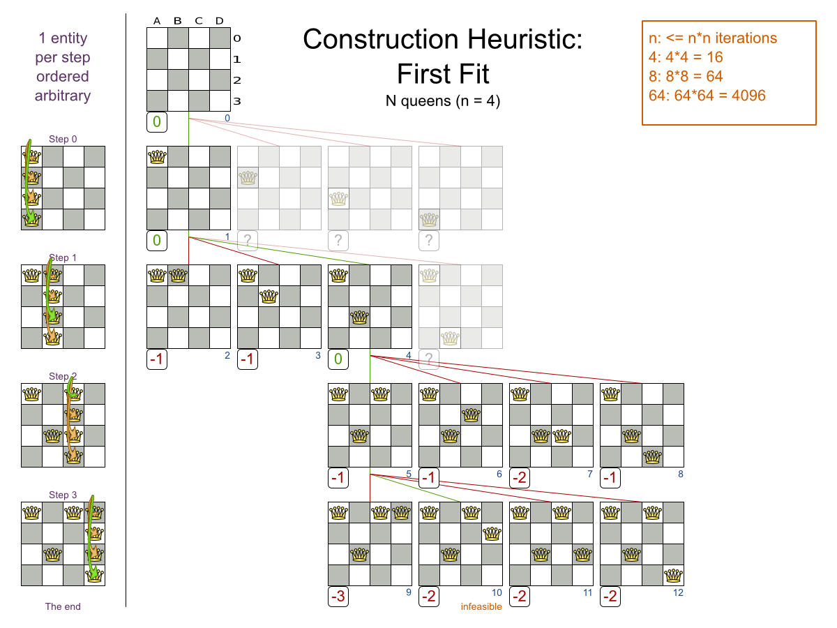
Notice that it starts with putting Queen A into row 0 (and never moving it later), which
makes it impossible to reach the optimal solution. Suffixing this construction heuristic with metaheuristics can
remedy that.
Configure this solver phase:
<constructionHeuristic>
<constructionHeuristicType>FIRST_FIT</constructionHeuristicType>
</constructionHeuristic>Note
If the InitializingScoreTrend is
ONLY_DOWN, this algorithm is faster: for an entity, it picks the first move for which the
score does not deteriorate the last step score, ignoring all subsequent moves.
For advanced configuration, see Allocate Entity From Queue.
Like First Fit, but assigns the more difficult planning entities first, because they are less likely to fit in the leftovers. So it sorts the planning entities on decreasing difficulty.
Requires the model to support planning entity difficulty comparison.
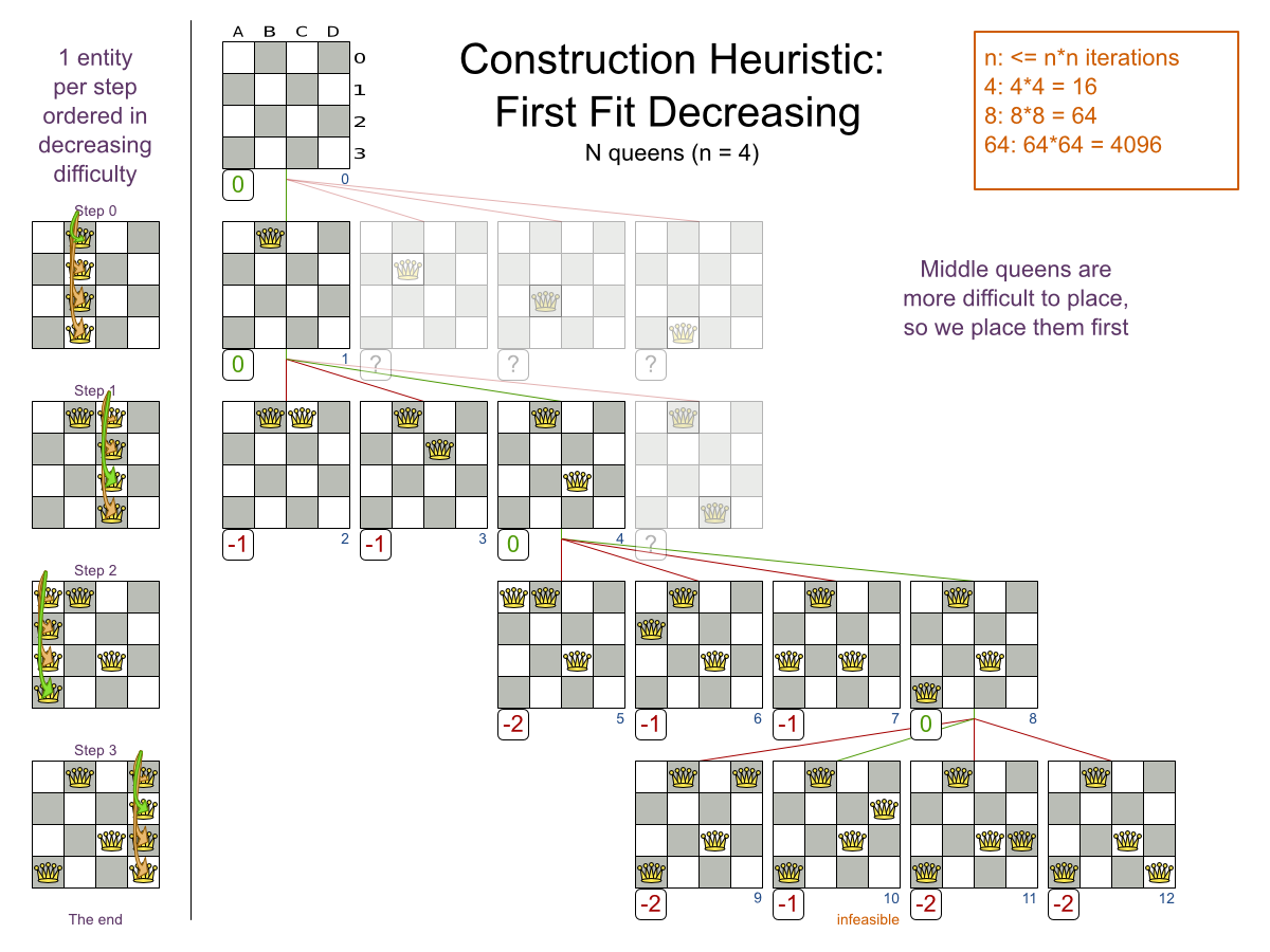
Note
One would expect that this algorithm has better results than First Fit. That's usually the case, but not always.
Configure this solver phase:
<constructionHeuristic>
<constructionHeuristicType>FIRST_FIT_DECREASING</constructionHeuristicType>
</constructionHeuristic>Note
If the InitializingScoreTrend is
ONLY_DOWN, this algorithm is faster: for an entity, it picks the first move for which the
score does not deteriorate the last step score, ignoring all subsequent moves.
For advanced configuration, see Allocate Entity From Queue.
Like First Fit, but uses the weaker planning values first, because the strong planning values are more likely to be able to accommodate later planning entities. So it sorts the planning values on increasing strength.
Requires the model to support planning value strength comparison.
Note
Do not presume that this algorithm has better results than First Fit. That's often not the case.
Configure this solver phase:
<constructionHeuristic>
<constructionHeuristicType>WEAKEST_FIT</constructionHeuristicType>
</constructionHeuristic>Note
If the InitializingScoreTrend is
ONLY_DOWN, this algorithm is faster: for an entity, it picks the first move for which the
score does not deteriorate the last step score, ignoring all subsequent moves.
For advanced configuration, see Allocate Entity From Queue.
Combines First Fit Decreasing and Weakest Fit. So it sorts the planning entities on decreasing difficulty and the planning values on increasing strength.
Requires the model to support planning entity difficulty comparison and planning value strength comparison.
Note
Do not presume that this algorithm has better results than First Fit Decreasing. That's often not the case. However, it is usually better than Weakest Fit.
Configure this solver phase:
<constructionHeuristic>
<constructionHeuristicType>WEAKEST_FIT_DECREASING</constructionHeuristicType>
</constructionHeuristic>Note
If the InitializingScoreTrend is
ONLY_DOWN, this algorithm is faster: for an entity, it picks the first move for which the
score does not deteriorate the last step score, ignoring all subsequent moves.
For advanced configuration, see Allocate Entity From Queue.
Like First Fit, but uses the strong planning values first, because the strong planning values are more likely to have a lower soft cost to use. So it sorts the planning values on decreasing strength.
Requires the model to support planning value strength comparison.
Note
Do not presume that this algorithm has better results than First Fit or Weakest Fit. That's often not the case.
Configure this solver phase:
<constructionHeuristic>
<constructionHeuristicType>STRONGEST_FIT</constructionHeuristicType>
</constructionHeuristic>Note
If the InitializingScoreTrend is
ONLY_DOWN, this algorithm is faster: for an entity, it picks the first move for which the
score does not deteriorate the last step score, ignoring all subsequent moves.
For advanced configuration, see Allocate Entity From Queue.
Combines First Fit Decreasing and Strongest Fit. So it sorts the planning entities on decreasing difficulty and the planning values on decreasing strength.
Requires the model to support planning entity difficulty comparison and planning value strength comparison.
Note
Do not presume that this algorithm has better results than First Fit Decreasing or Weakest Fit Decreasing. That's often not the case. However, it is usually better than Strongest Fit.
Configure this solver phase:
<constructionHeuristic>
<constructionHeuristicType>STRONGEST_FIT_DECREASING</constructionHeuristicType>
</constructionHeuristic>Note
If the InitializingScoreTrend is
ONLY_DOWN, this algorithm is faster: for an entity, it picks the first move for which the
score does not deteriorate the last step score, ignoring all subsequent moves.
For advanced configuration, see Allocate Entity From Queue.
Allocate Entity From Queue is a versatile, generic form of First Fit, First Fit Decreasing, Weakest Fit and Weakest Fit Decreasing. It works like this:
Put all entities in a queue.
Assign the first entity (from that queue) to the best value.
Repeat until all entities are assigned.
Simple configuration:
<constructionHeuristic>
<constructionHeuristicType>ALLOCATE_ENTITY_FROM_QUEUE</constructionHeuristicType>
</constructionHeuristic>Verbose simple configuration:
<constructionHeuristic>
<constructionHeuristicType>ALLOCATE_ENTITY_FROM_QUEUE</constructionHeuristicType>
<entitySorterManner>DECREASING_DIFFICULTY_IF_AVAILABLE</entitySorterManner>
<valueSorterManner>INCREASING_STRENGTH_IF_AVAILABLE</valueSorterManner>
</constructionHeuristic>The entitySorterManner options are:
DECREASING_DIFFICULTY: Initialize the more difficult planning entities first. This usually increases pruning (and therefore improves scalability). Requires the model to support planning entity difficulty comparison.DECREASING_DIFFICULTY_IF_AVAILABLE(default): If the model supports planning entity difficulty comparison, behave likeDECREASING_DIFFICULTY, else likeNONE.NONE: Initialize the planning entities in original order.
The valueSorterManner options are:
INCREASING_STRENGTH: Evaluate the planning values in increasing strength. Requires the model to support planning value strength comparison.INCREASING_STRENGTH_IF_AVAILABLE(default): If the model supports planning value strength comparison, behave likeINCREASING_STRENGTH, else likeNONE.DECREASING_STRENGTH: Evaluate the planning values in decreasing strength. Requires the model to support planning value strength comparison.DECREASING_STRENGTH_IF_AVAILABLE: If the model supports planning value strength comparison, behave likeDECREASING_STRENGTH, else likeNONE.NONE: Try the planning values in original order.
Advanced detailed configuration. For example, a Weakest Fit Decreasing configuration for a single entity class with a single variable:
<constructionHeuristic>
<queuedEntityPlacer>
<entitySelector id="placerEntitySelector">
<cacheType>PHASE</cacheType>
<selectionOrder>SORTED</selectionOrder>
<sorterManner>DECREASING_DIFFICULTY</sorterManner>
</entitySelector>
<changeMoveSelector>
<entitySelector mimicSelectorRef="placerEntitySelector"/>
    <valueSelector>
      <cacheType>PHASE</cacheType>
      <selectionOrder>SORTED</selectionOrder>
      <sorterManner>INCREASING_STRENGTH</sorterManner>
    </valueSelector>
</changeMoveSelector>
</queuedEntityPlacer>
</constructionHeuristic>Per step, the QueuedEntityPlacer selects 1 uninitialized entity from the
EntitySelector and applies the winning Move (out of all the moves for that
entity generated by the MoveSelector). The mimic
selection ensures that the winning Move changes (only) the selected entity.
To customize the entity or value sorting, see sorted selection. Other
Selector customization (such as filtering and limiting) is supported too.
There are 2 ways to deal with multiple variables, depending on how their ChangeMoves are
combined:
Cartesian product of the
ChangeMoves (default): All variables of the selected entity are assigned together. Has far better results (especially for timetabling use cases).Sequential
ChangeMoves: One variable is assigned at a time. Scales much better, especially for 3 or more variables.
For example, presume a course scheduling example with 200 rooms and 40 periods.
This First Fit configuration for a single entity class with 2 variables, using a cartesian product of their ChangeMoves, will
select 8000 moves per entity:
<constructionHeuristic>
<queuedEntityPlacer>
<entitySelector id="placerEntitySelector">
<cacheType>PHASE</cacheType>
</entitySelector>
<cartesianProductMoveSelector>
<changeMoveSelector>
<entitySelector mimicSelectorRef="placerEntitySelector"/>
<valueSelector>
<variableName>room</variableName>
</valueSelector>
</changeMoveSelector>
<changeMoveSelector>
<entitySelector mimicSelectorRef="placerEntitySelector"/>
<valueSelector>
<variableName>period</variableName>
</valueSelector>
</changeMoveSelector>
</cartesianProductMoveSelector>
</queuedEntityPlacer>
...
</constructionHeuristic>Warning
With 3 variables of 1000 values each, a cartesian product selects 1000000000 values per entity, which will take far too long.
This First Fit configuration for a single entity class with 2 variables, using sequential
ChangeMoves, will select 240 moves per entity:
<constructionHeuristic>
<queuedEntityPlacer>
<entitySelector id="placerEntitySelector">
<cacheType>PHASE</cacheType>
</entitySelector>
<changeMoveSelector>
<entitySelector mimicSelectorRef="placerEntitySelector"/>
<valueSelector>
<variableName>period</variableName>
</valueSelector>
</changeMoveSelector>
<changeMoveSelector>
<entitySelector mimicSelectorRef="placerEntitySelector"/>
<valueSelector>
<variableName>room</variableName>
</valueSelector>
</changeMoveSelector>
</queuedEntityPlacer>
...
</constructionHeuristic>Important
Especially for sequential ChangeMoves, the order of the variables is important. In the
example above, it's better to select the period first (instead of the other way around), because there are more
hard constraints that do not involve the room (for example: no teacher should teach 2 lectures at the same
time). Let the Benchmarker guide you.
With 3 or more variables, it's possible to combine the cartesian product and sequential techniques:
<constructionHeuristic>
<queuedEntityPlacer>
...
<cartesianProductMoveSelector>
<changeMoveSelector>...</changeMoveSelector>
<changeMoveSelector>...</changeMoveSelector>
</cartesianProductMoveSelector>
<changeMoveSelector>...</changeMoveSelector>
</queuedEntityPlacer>
...
</constructionHeuristic>The easiest way to deal with multiple entity classes is to run a separate construction heuristic for each entity class:
<constructionHeuristic>
<queuedEntityPlacer>
<entitySelector id="placerEntitySelector">
<cacheType>PHASE</cacheType>
<entityClass>...DogEntity</entityClass>
</entitySelector>
<changeMoveSelector>
<entitySelector mimicSelectorRef="placerEntitySelector"/>
</changeMoveSelector>
</queuedEntityPlacer>
...
</constructionHeuristic>
<constructionHeuristic>
<queuedEntityPlacer>
<entitySelector id="placerEntitySelector">
<cacheType>PHASE</cacheType>
<entityClass>...CatEntity</entityClass>
</entitySelector>
<changeMoveSelector>
<entitySelector mimicSelectorRef="placerEntitySelector"/>
</changeMoveSelector>
</queuedEntityPlacer>
...
</constructionHeuristic>There are several pick early types for Construction Heuristics:
NEVER: Evaluate all the selected moves to initialize the variable(s). This is the default if the InitializingScoreTrend is notONLY_DOWN.<constructionHeuristic> ... <forager> <pickEarlyType>NEVER</pickEarlyType> </forager> </constructionHeuristic>FIRST_NON_DETERIORATING_SCORE: Initialize the variable(s) with the first move that doesn't deteriorate the score, ignore the remaining selected moves. This is the default if the InitializingScoreTrend isONLY_DOWN.<constructionHeuristic> ... <forager> <pickEarlyType>FIRST_NON_DETERIORATING_SCORE</pickEarlyType> </forager> </constructionHeuristic>Note
If there are only negative constraints, but the InitializingScoreTrend is strictly not
ONLY_DOWN, it can sometimes make sense to apply FIRST_NON_DETERIORATING_SCORE. Use the Benchmarker to decide if the score quality loss is worth the time gain.FIRST_FEASIBLE_SCORE: Initialize the variable(s) with the first move that has a feasible score.<constructionHeuristic> ... <forager> <pickEarlyType>FIRST_FEASIBLE_SCORE</pickEarlyType> </forager> </constructionHeuristic>If the InitializingScoreTrend is
ONLY_DOWN, useFIRST_FEASIBLE_SCORE_OR_NON_DETERIORATING_HARDinstead, because that's faster without any disadvantages.FIRST_FEASIBLE_SCORE_OR_NON_DETERIORATING_HARD: Initialize the variable(s) with the first move that doesn't deteriorate the feasibility of the score any further.<constructionHeuristic> ... <forager> <pickEarlyType>FIRST_FEASIBLE_SCORE_OR_NON_DETERIORATING_HARD</pickEarlyType> </forager> </constructionHeuristic>
Allocate To Value From Queue is a versatile, generic form of Nearest Neighbour. It works like this:
Put all values in a round-robin queue.
Assign the best entity to the first value (from that queue).
Repeat until all entities are assigned.
The Cheapest Insertion algorithm cycles through all the planning values for all the planning entities, initializing 1 planning entity at a time. It assigns a planning entity to the best available planning value (out of all the planning entities and values), taking the already initialized planning entities into account. It terminates when all planning entities have been initialized. It never changes a planning entity after it has been assigned.
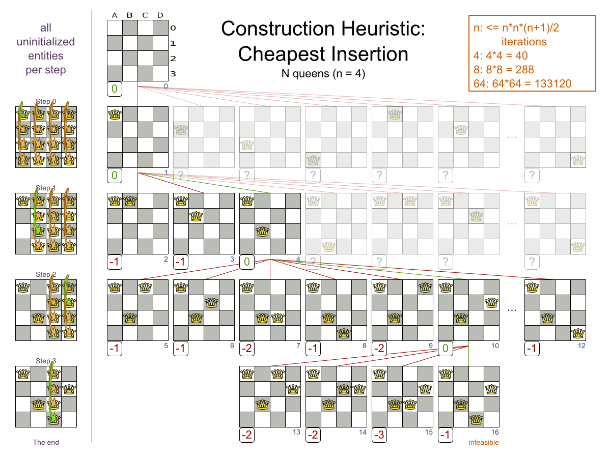
Note
Cheapest Insertion scales considerably worse than First Fit, etc.
Simplest configuration of Cheapest Insertion:
<constructionHeuristic>
<constructionHeuristicType>CHEAPEST_INSERTION</constructionHeuristicType>
</constructionHeuristic>Note
If the InitializingScoreTrend is
ONLY_DOWN, this algorithm is faster: for an entity, it picks the first move for which the
score does not deteriorate the last step score, ignoring all subsequent moves.
For advanced configuration, see Allocate from pool.
The Regret Insertion algorithm behaves like the Cheapest Insertion algorithm. It also cycles through all the planning values for all the planning entities, initializing 1 planning entity at a time. But instead of picking the entity-value combination with the best score, it picks the entity which has the largest score loss between its best and second best value assignment. It then assigns that entity to its best value, to avoid regretting not having done that.
Allocate From Pool is a versatile, generic form of Cheapest Insertion and Regret Insertion. It works like this:
Put all entity-value combinations in a pool.
Assign the best entity to best value.
Repeat until all entities are assigned.
Simple configuration:
<constructionHeuristic>
<constructionHeuristicType>ALLOCATE_FROM_POOL</constructionHeuristicType>
</constructionHeuristic>Verbose simple configuration:
<constructionHeuristic>
<constructionHeuristicType>ALLOCATE_FROM_POOL</constructionHeuristicType>
<entitySorterManner>DECREASING_DIFFICULTY_IF_AVAILABLE</entitySorterManner>
<valueSorterManner>INCREASING_STRENGTH_IF_AVAILABLE</valueSorterManner>
</constructionHeuristic>The entitySorterManner and valueSorterManner options are described in
Allocate Entity From Queue.
Advanced detailed configuration. For example, a Cheapest Insertion configuration for a single entity class with a single variable:
<constructionHeuristic>
<pooledEntityPlacer>
<changeMoveSelector>
<entitySelector id="placerEntitySelector">
<cacheType>PHASE</cacheType>
<selectionOrder>SORTED</selectionOrder>
<sorterManner>DECREASING_DIFFICULTY</sorterManner>
</entitySelector>
<valueSelector>
<cacheType>PHASE</cacheType>
<selectionOrder>SORTED</selectionOrder>
<sorterManner>INCREASING_STRENGTH</sorterManner>
</valueSelector>
</changeMoveSelector>
</pooledEntityPlacer>
</constructionHeuristic>Per step, the PooledEntityPlacer applies the winning Move (out of all
the moves for that entity generated by the MoveSelector).
To customize the entity or value sorting, see sorted selection. Other
Selector customization (such as filtering and limiting) is supported too.
Local Search starts from an initial solution and evolves that single solution into a mostly better and better solution. It uses a single search path of solutions, not a search tree. At each solution in this path it evaluates a number of moves on the solution and applies the most suitable move to take the step to the next solution. It does that for a high number of iterations until it's terminated (usually because its time has run out).
Local Search acts a lot like a human planner: it uses a single search path and moves facts around to find a good feasible solution. Therefore it's pretty natural to implement.
Local Search usually needs to start from an initialized solution, therefore it's usually required to configure a construction heuristic solver phase before it.
A step is the winning Move. Local Search tries a number of moves on the current solution
and picks the best accepted move as the step:
Because the move B0 to B3 has the highest score (-3), it is picked
as the next step. If multiple moves have the same highest score, one is picked randomly, in this case B0
to B3. Note that C0 to C3 (not shown) could also have been picked because it also
has the score -3.
The step is applied on the solution. From that new solution, Local Search tries every move again, to decide the next step after that. It continually does this in a loop, and we get something like this:
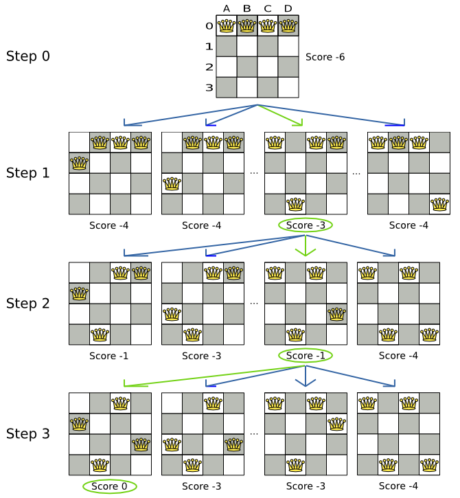
Notice that Local Search doesn't use a search tree, but a search path. The search path is highlighted by the green arrows. At each step it tries all selected moves, but unless it's the step, it doesn't investigate that solution further. This is one of the reasons why Local Search is very scalable.
As shown above, Local Search solves the 4 queens problem by starting with the starting solution and make the following steps sequentially:
B0 to B3
D0 to B2
A0 to B1
Turn on debug logging for the category org.optaplanner to show those
steps in the log:
INFO Solving started: time spent (0), best score (-6), random (JDK with seed 0).
DEBUG LS step (0), time spent (20), score (-3), new best score (-3), accepted/selected move count (12/12), picked move (Queen-1 {Row-0 -> Row-3}).
DEBUG LS step (1), time spent (31), score (-1), new best score (-1), accepted/selected move count (12/12), picked move (Queen-3 {Row-0 -> Row-2}).
DEBUG LS step (2), time spent (40), score (0), new best score (0), accepted/selected move count (12/12), picked move (Queen-0 {Row-0 -> Row-1}).
INFO Local Search phase (0) ended: step total (3), time spent (41), best score (0).
INFO Solving ended: time spent (41), best score (0), average calculate count per second (1780).Notice that a log message includes the toString() method of the Move
implementation which returns for example "Queen-1 {Row-0 -> Row-3}".
A naive Local Search configuration solves the 4 queens problem in 3 steps, by evaluating only 37 possible solutions (3 steps with 12 moves each + 1 starting solution), which is only fraction of all 256 possible solutions. It solves 16 queens in 31 steps, by evaluating only 7441 out of 18446744073709551616 possible solutions. By using a Construction Heuristics phase first, it's even a lot more efficient.
Local Search decides the next step with the aid of 3 configurable components:
A
MoveSelectorwhich selects the possible moves of the current solution. See the chapter move and neighborhood selection.An
Acceptorwhich filters out unacceptable moves.A
Foragerwhich gathers accepted moves and picks the next step from them.
The solver phase configuration looks like this:
<localSearch>
<unionMoveSelector>
...
</unionMoveSelector>
<acceptor>
...
</acceptor>
<forager>
...
</forager>
</localSearch>In the example below, the MoveSelector generated the moves shown with the blue lines, the
Acceptor accepted all of them and the Forager picked the move B0
to B3.
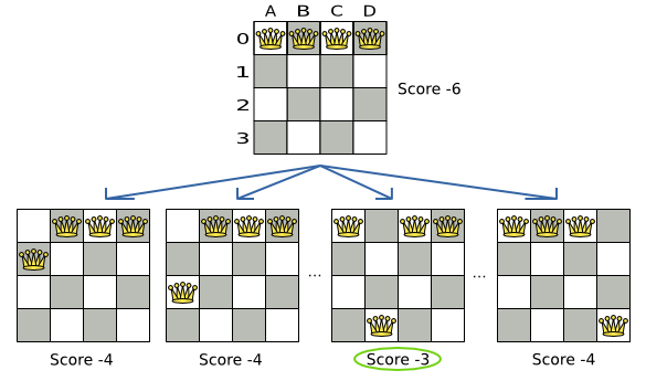
Turn on trace logging to show the decision making in the
log:
INFO Solver started: time spent (0), score (-6), new best score (-6), random (JDK with seed 0).
TRACE Move index (0) not doable, ignoring move (Queen-0 {Row-0 -> Row-0}).
TRACE Move index (1), score (-4), accepted (true), move (Queen-0 {Row-0 -> Row-1}).
TRACE Move index (2), score (-4), accepted (true), move (Queen-0 {Row-0 -> Row-2}).
TRACE Move index (3), score (-4), accepted (true), move (Queen-0 {Row-0 -> Row-3}).
...
TRACE Move index (6), score (-3), accepted (true), move (Queen-1 {Row-0 -> Row-3}).
...
TRACE Move index (9), score (-3), accepted (true), move (Queen-2 {Row-0 -> Row-3}).
...
TRACE Move index (12), score (-4), accepted (true), move (Queen-3 {Row-0 -> Row-3}).
DEBUG LS step (0), time spent (6), score (-3), new best score (-3), accepted/selected move count (12/12), picked move (Queen-1 {Row-0 -> Row-3}).
...Because the last solution can degrade (for example in Tabu Search), the Solver remembers
the best solution it has encountered through the entire search path. Each time the current solution is better than
the last best solution, the current solution is cloned and referenced as
the new best solution.
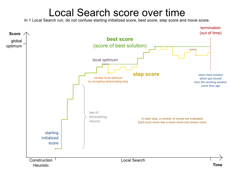
An Acceptor is used (together with a Forager) to active Tabu Search,
Simulated Annealing, Late Acceptance, ... For each move it checks whether it is accepted or not.
By changing a few lines of configuration, you can easily switch from Tabu Search to Simulated Annealing or Late Acceptance and back.
You can implement your own Acceptor, but the build-in acceptors should suffice for most
needs. You can also combine multiple acceptors.
A Forager gathers all accepted moves and picks the move which is the next step. Normally
it picks the accepted move with the highest score. If several accepted moves have the highest score, one is picked
randomly to break the tie. Breaking ties randomly leads to better results.
Note
It is possible to disable breaking ties randomly by explicitly setting breakTieRandomly
to false, but that's almost never a good idea:
If an earlier move is better than a later move with the same score, the score calculator should add an extra softer score level to score the first move as slightly better. Don't rely on move selection order to enforce that.
Random tie breaking does not affect reproducibility.
When there are many possible moves, it becomes inefficient to evaluate all of them at every step. To evaluate only a random subset of all the moves, use:
An
acceptedCountLimitinteger, which specifies how many accepted moves should be evaluated during each step. By default, all accepted moves are evaluated at every step.<forager> <acceptedCountLimit>1000</acceptedCountLimit> </forager>
Unlike the n queens problem, real world problems require the use of acceptedCountLimit.
Start from an acceptedCountLimit that takes a step in less then 2 seconds. Turn on INFO logging to see the step times. Use the Benchmarker to tweak the value.
Important
With a low acceptedCountLimit (so a fast stepping algorithm), it is recommended to
avoid using selectionOrder SHUFFLED because the shuffling generates a random number for
every element in the selector, taking up a lot of time, but only a few elements are actually selected.
A forager can pick a move early during a step, ignoring subsequent selected moves. There are 3 pick early types for Local Search:
NEVER: A move is never picked early: all accepted moves are evaluated that the selection allows. This is the default.<forager> <pickEarlyType>NEVER</pickEarlyType> </forager>FIRST_BEST_SCORE_IMPROVING: Pick the first accepted move that improves the best score. If none improve the best score, it behaves exactly like the pickEarlyType NEVER.<forager> <pickEarlyType>FIRST_BEST_SCORE_IMPROVING</pickEarlyType> </forager>FIRST_LAST_STEP_SCORE_IMPROVING: Pick the first accepted move that improves the last step score. If none improve the last step score, it behaves exactly like the pickEarlyType NEVER.<forager> <pickEarlyType>FIRST_LAST_STEP_SCORE_IMPROVING</pickEarlyType> </forager>
Hill Climbing tries all selected moves and then takes the best move, which is the move which leads to the solution with the highest score. That best move is called the step move. From that new solution, it again tries all selected moves and takes the best move and continues like that iteratively. If multiple selected moves tie for the best move, one of them is randomly chosen as the best move.
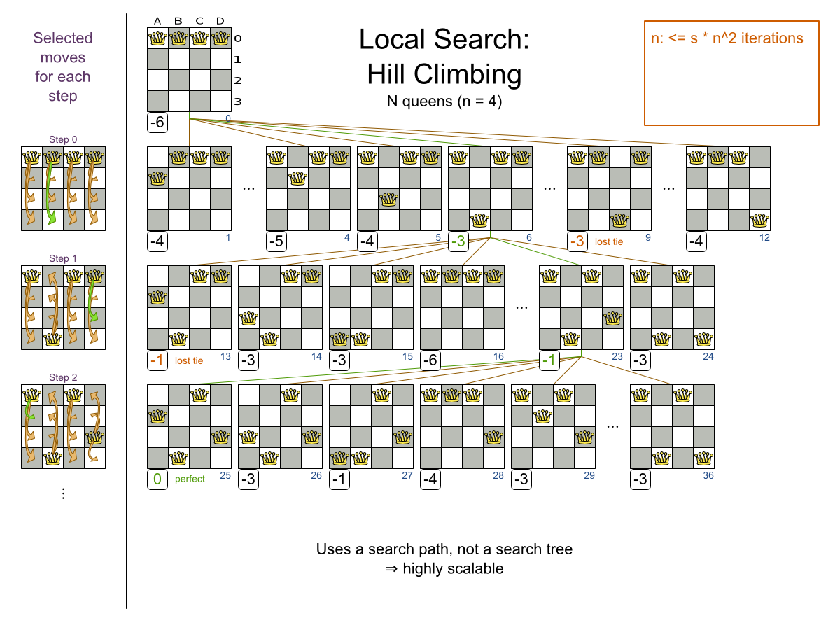
Notice that once a queen has moved, it can be moved again later. This is a good thing, because in an NP-complete problem it's impossible to predict what will be the optimal final value for a planning variable.
Hill Climbing always takes improving moves. This may seem like a good thing, but it's not: Hill Climbing can easily get stuck in a local optimum. This happens when it reaches a solution for which all the moves deteriorate the score. Even if it picks one of those moves, the next step might go back to the original solution and which case chasing its own tail:
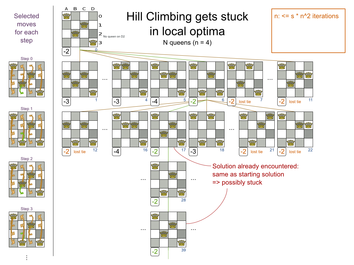
Improvements upon Hill Climbing (such as Tabu Search, Simulated Annealing and Late Acceptance) address the problem of being stuck in local optima. Therefore, it's recommend to never use Hill Climbing, unless you're absolutely sure there are no local optima in your planning problem.
Simplest configuration:
<localSearch>
<localSearchType>HILL_CLIMBING</localSearchType>
</localSearch>Advanced configuration:
<localSearch>
...
<acceptor>
<acceptorType>HILL_CLIMBING</acceptorType>
</acceptor>
<forager>
<acceptedCountLimit>1</acceptedCountLimit>
</forager>
</localSearch>Tabu Search works like Hill Climbing, but it maintains a tabu list to avoid getting stuck in local optima. The tabu list holds recently used objects that are taboo to use for now. Moves that involve an object in the tabu list, are not accepted. The tabu list objects can be anything related to the move, such as the planning entity, planning value, move, solution, ... Here's an example with entity tabu for 4 queens, so the queens are put in the tabu list:
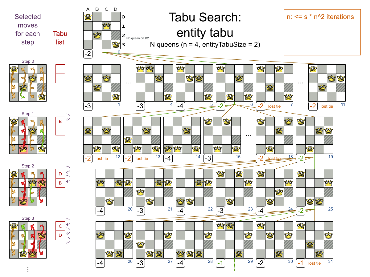
Note
It's called Tabu Search, not Taboo Search. There is no spelling error.
Scientific paper: Tabu Search - Part 1 and Part 2 by Fred Glover (1989 - 1990)
Simplest configuration:
<localSearch>
<localSearchType>TABU_SEARCH</localSearchType>
</localSearch>When Tabu Search takes steps it creates one or more tabu's. For a number of steps, it does not accept a move if that move breaks tabu. That number of steps is the tabu size. Advanced configuration:
<localSearch>
...
<acceptor>
<entityTabuSize>7</entityTabuSize>
</acceptor>
<forager>
<acceptedCountLimit>1000</acceptedCountLimit>
</forager>
</localSearch>Important
A Tabu Search acceptor should be combined with a high acceptedCountLimit, such as
1000.
Planner implements several tabu types:
Planning entity tabu (recommended) makes the planning entities of recent steps tabu. For example, for N queens it makes the recently moved queens tabu. It's recommended to start with this tabu type.
<acceptor> <entityTabuSize>7</entityTabuSize> </acceptor>To avoid hard coding the tabu size, configure a tabu ratio, relative to the number of entities, for example 2%:
<acceptor> <entityTabuRatio>0.02</entityTabuRatio> </acceptor>Planning value tabu makes the planning values of recent steps tabu. For example, for N queens it makes the recently moved to rows tabu.
<acceptor> <valueTabuSize>7</valueTabuSize> </acceptor>To avoid hard coding the tabu size, configure a tabu ratio, relative to the number of values, for example 2%:
<acceptor> <valueTabuRatio>0.02</valueTabuRatio> </acceptor>Move tabu makes recent steps tabu. It does not accept a move equal to one of those steps.
<acceptor> <moveTabuSize>7</moveTabuSize> </acceptor>Undo move tabu makes the undo move of recent steps tabu.
<acceptor> <undoMoveTabuSize>7</undoMoveTabuSize> </acceptor>Solution tabu makes recently visited solutions tabu. It does not accept a move that leads to one of those solutions. It requires that the
Solutionimplementsequals()andhashCode()properly. If you can spare the memory, don't be cheap on the tabu size.<acceptor> <solutionTabuSize>1000</solutionTabuSize> </acceptor>For non-trivial cases, solution tabu is usually useless because the search space size makes it statistically highly unlikely to reach the same solution twice. Therefore its use is not recommended, except for small datasets.
Sometimes it's useful to combine tabu types:
<acceptor>
<entityTabuSize>7</entityTabuSize>
<valueTabuSize>3</valueTabuSize>
</acceptor>If the tabu size is too small, the solver can still get stuck in a local optimum. On the other hand, if the tabu size is too large, the solver can be inefficient by bouncing of the walls. Use the Benchmarker to fine tweak your configuration.
Simulated Annealing evaluates only a few moves per step, so it steps quickly. In the classic implementation, the first accepted move is the winning step. A move is accepted if it doesn't decrease the score or - in case it does decrease the score - it passes a random check. The chance that a decreasing move passes the random check decreases relative to the size of the score decrement and the time the phase has been running (which is represented as the temperature).
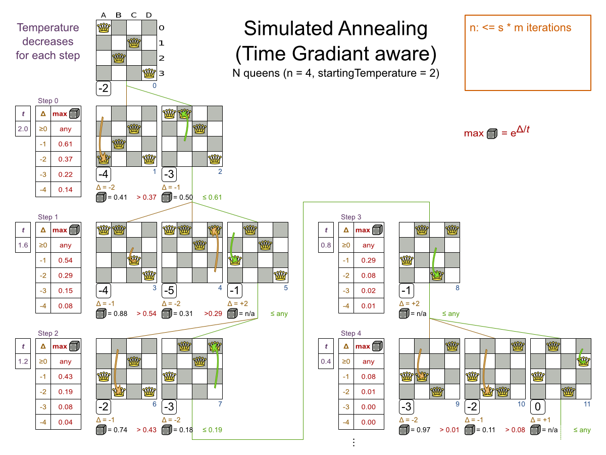
Simulated Annealing does not always pick the move with the highest score, neither does it evaluate many
moves per step. At least at first. Instead, it gives non improving moves also a chance to be picked, depending on
its score and the time gradient of the Termination. In the end, it gradually turns into Hill
Climbing, only accepting improving moves.
Start with a simulatedAnnealingStartingTemperature set to the maximum score delta a
single move can cause. Use the Benchmarker to tweak the value. Advanced
configuration:
<localSearch>
...
<acceptor>
<simulatedAnnealingStartingTemperature>2hard/100soft</simulatedAnnealingStartingTemperature>
</acceptor>
<forager>
<acceptedCountLimit>1</acceptedCountLimit>
</forager>
</localSearch>Simulated Annealing should use a low acceptedCountLimit. The classic algorithm uses an
acceptedCountLimit of 1, but often 4 performs
better.
Simulated Annealing can be combined with a tabu acceptor at the same time. That gives Simulated Annealing salted with a bit of Tabu. Use a lower tabu size than in a pure Tabu Search configuration.
<localSearch>
...
<acceptor>
<simulatedAnnealingStartingTemperature>2hard/100soft</simulatedAnnealingStartingTemperature>
<entityTabuSize>5</entityTabuSize>
</acceptor>
<forager>
<acceptedCountLimit>1</acceptedCountLimit>
</forager>
</localSearch>Late Acceptance (also known as Late Acceptance Hill Climbing) also evaluates only a few moves per step. A move is accepted if it does not decrease the score, or if it leads to a score that is at least the late score (which is the winning score of a fixed number of steps ago).
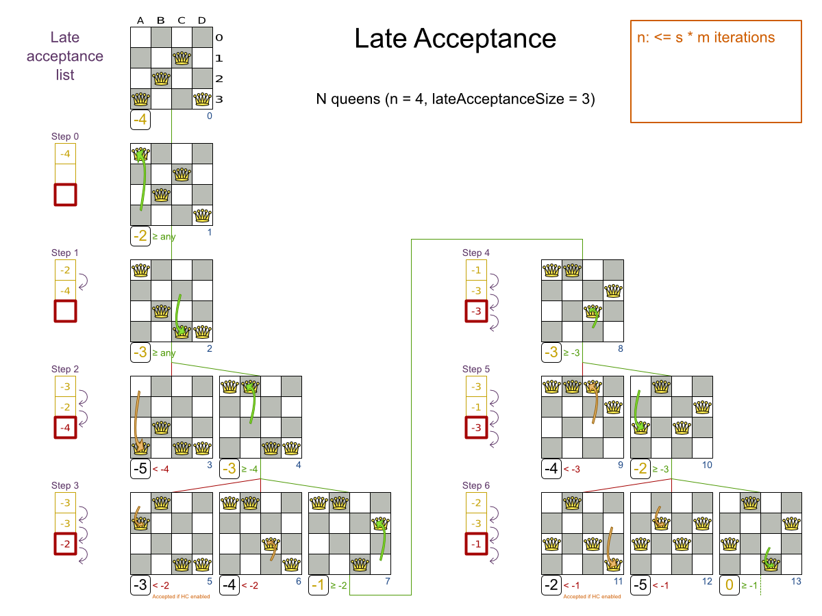
Scientific paper: The Late Acceptance Hill-Climbing Heuristic by Edmund K. Burke, Yuri Bykov (2012)
Simplest configuration:
<localSearch>
<localSearchType>LATE_ACCEPTANCE</localSearchType>
</localSearch>Late Acceptance accepts any move that has a score which is higher than the best score of a number of steps
ago. That number of steps is the lateAcceptanceSize. Advanced configuration:
<localSearch>
...
<acceptor>
<lateAcceptanceSize>400</lateAcceptanceSize>
</acceptor>
<forager>
<acceptedCountLimit>1</acceptedCountLimit>
</forager>
</localSearch>Late Acceptance should use a low acceptedCountLimit.
Late Acceptance can be combined with a tabu acceptor at the same time. That gives Late Acceptance salted with a bit of Tabu. Use a lower tabu size than in a pure Tabu Search configuration.
<localSearch>
...
<acceptor>
<lateAcceptanceSize>400</lateAcceptanceSize>
<entityTabuSize>5</entityTabuSize>
</acceptor>
<forager>
<acceptedCountLimit>1</acceptedCountLimit>
</forager>
</localSearch>Step Counting Hill Climbing also evaluates only a few moves per step. For a number of steps, it keeps the step score as a threshold. A move is accepted if it does not decrease the score, or if it leads to a score that is at least the threshold score.
Scientific paper: An initial study of a novel Step Counting Hill Climbing heuristic applied to timetabling problems by Yuri Bykov, Sanja Petrovic (2013)
Step Counting Hill Climbing accepts any move that has a score which is higher than a threshold score. Every
number of steps (specified by stepCountingHillClimbingSize), the threshold score is set to the
step score.
<localSearch>
...
<acceptor>
<stepCountingHillClimbingSize>400</stepCountingHillClimbingSize>
</acceptor>
<forager>
<acceptedCountLimit>1</acceptedCountLimit>
</forager>
</localSearch>Step Counting Hill Climbing should use a low acceptedCountLimit.
Step Counting Hill Climbing can be combined with a tabu acceptor at the same time, similar as shown in the Late Acceptance section.
Strategic Oscillation is an add-on, which works especially well with Tabu Search. Instead of picking the accepted move with the highest score, it employs a different mechanism: If there's an improving move, it picks it. If there's no improving move however, it prefers moves which improve a softer score level, over moves which break a harder score level less.
Configure a finalistPodiumType, for example in a Tabu Search configuration:
<localSearch>
...
<acceptor>
<entityTabuSize>7</entityTabuSize>
</acceptor>
<forager>
<acceptedCountLimit>1000</acceptedCountLimit>
<finalistPodiumType>STRATEGIC_OSCILLATION</finalistPodiumType>
</forager>
</localSearch>The following finalistPodiumTypes are supported:
HIGHEST_SCORE(default): Pick the accepted move with the highest score.STRATEGIC_OSCILLATION: Alias for the default strategic oscillation variant.STRATEGIC_OSCILLATION_BY_LEVEL: If there is an accepted improving move, pick it. If no such move exists, prefer an accepted move which improves a softer score level over one that doesn't (even if it has a better harder score level). A move is improving if it's better than the last completed step score.STRATEGIC_OSCILLATION_BY_LEVEL_ON_BEST_SCORE: LikeSTRATEGIC_OSCILLATION_BY_LEVEL, but define improving as better than the best score (instead of the last completed step score).
You can plug in a custom Termination, MoveSelector,
EntitySelector, ValueSelector or Acceptor by extending the
abstract class and also the related *Config class.
For example, to use a custom MoveSelector, extend the
AbstractMoveSelector class, extend the MoveSelectorConfig class and configure
it in the solver configuration.
Note
It's not possible to inject a Termination, ... instance directly (to avoid extending a
Config class too) because:
A
SolverFactorycan build multipleSolverinstances, which each require a distinctTermination, ... instance.A solver configuration needs to be serializable to and from XML. This makes benchmarking with
PlannerBenchmarkparticularly easy because you can configure differentSolvervariants in XML.A
Configclass is often easier and clearer to configure. For example:TerminationConfigtranslatesminutesSpentLimitandsecondsSpentLimitintotimeMillisSpentLimit.
If you build a better implementation that's not domain specific, consider contributing it back as a pull request on github: we'll optimize it and take it along in future refactorings.
This algorithm has not been implemented yet.
Note
A good Genetic Algorithms prototype in Planner was written some time ago, but it wasn't practical to merge and support it at the time. The results of Genetic Algorithms were consistently and seriously inferior to all the Local Search variants (except Hill Climbing) on all use cases tried. Nevertheless, a future version of Planner will add support for Genetic Algorithms, so you can easily benchmark Genetic Algorithms on your use case too.
A hyperheuristic automates the decision which heuristic(s) to use on a specific data set.
A future version of Planner will have native support for hyperheuristics. Meanwhile, it's pretty easy to implement it yourself: Based on the size or difficulty of a data set (which is a criterion), use a different Solver configuration (or adjust the default configuration using the Solver configuration API). The Benchmarker can help to identify such criteria.
For very big datasets, it is sometimes worthwhile to partition the datasets into smaller pieces.
However, partitioning leads to suboptimal results, even if the pieces are solved optimally:
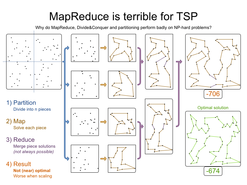
A future version of Planner will have native support for several forms of partitioning. Meanwhile, you can
implement it yourself as shown in the image above. Use an Solver to solve each piece.
Note
Not all use cases can be partitioned. It only works on use cases for which the planning entities and value ranges can be divided into n pieces, such that none of the constraints cross piece boundaries.
- 14.1. Find The Best
SolverConfiguration - 14.2. Benchmark Configuration
- 14.2.1. Add Dependency On
optaplanner-benchmark - 14.2.2. Build And Run A
PlannerBenchmark - 14.2.3. SolutionFileIO: Input And Output Of Solution Files
- 14.2.4. Warming Up The HotSpot Compiler
- 14.2.5. Benchmark Blueprint: A Predefined Configuration
- 14.2.6. Write The Output Solution Of Benchmark Runs
- 14.2.7. Benchmark Logging
- 14.2.1. Add Dependency On
- 14.3. Benchmark Report
- 14.4. Summary Statistics
- 14.4.1. Best Score Summary (Graph And Table)
- 14.4.2. Best Score Scalability Summary (Graph)
- 14.4.3. Winning Score Difference Summary (Graph And Table)
- 14.4.4. Worst Score Difference Percentage (ROI) Summary (Graph and Table)
- 14.4.5. Average Calculation Count Summary (Graph and Table)
- 14.4.6. Time Spent Summary (Graph And Table)
- 14.4.7. Time Spent Scalability Summary (Graph)
- 14.4.8. Best Score Per Time Spent Summary (Graph)
- 14.5. Statistic Per Dataset (Graph And CSV)
- 14.5.1. Enable A Problem Statistic
- 14.5.2. Best Score Over Time Statistic (Graph And CSV)
- 14.5.3. Step Score Over Time Statistic (Graph And CSV)
- 14.5.4. Calculate Count Per Second Statistic (Graph And CSV)
- 14.5.5. Best Solution Mutation Over Time Statistic (Graph And CSV)
- 14.5.6. Move Count Per Step Statistic (Graph And CSV)
- 14.5.7. Memory Use Statistic (Graph And CSV)
- 14.6. Statistic Per Single Benchmark (Graph And CSV)
- 14.6.1. Enable A Single Statistic
- 14.6.2. Constraint Match Total Best Score Over Time Statistic (Graph And CSV)
- 14.6.3. Constraint Match Total Step Score Over Time Statistic (Graph And CSV)
- 14.6.4. Picked Move Type Best Score Diff Over Time Statistic (Graph And CSV)
- 14.6.5. Picked Move Type Step Score Diff Over Time Statistic (Graph And CSV)
- 14.7. Advanced Benchmarking
Planner supports several optimization algorithms, so you're probably wondering which is the best one? Although some optimization algorithms generally perform better than others, it really depends on your problem domain. Most solver phases have parameters which can be tweaked. Those parameters can influence the results a lot, even though most solver phases work pretty well out-of-the-box.
Luckily, Planner includes a benchmarker, which allows you to play out different solver phases with different settings against each other in development, so you can use the best configuration for your planning problem in production.
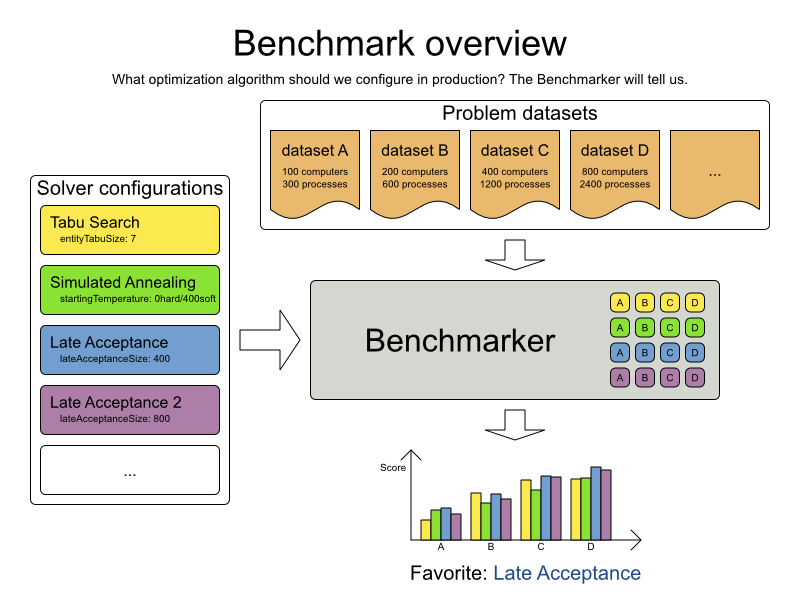
The benchmarker is in a separate artifact called optaplanner-benchmark.
If you use Maven, add a dependency in your pom.xml file:
<dependency>
<groupId>org.optaplanner</groupId>
<artifactId>optaplanner-benchmark</artifactId>
</dependency>This is similar for Gradle, Ivy and Buildr. The version must be exactly the same as the
optaplanner-core version used (which is automatically the case if you import
optaplanner-bom).
If you use ANT, you've probably already copied the required jars from the download zip's
binaries directory.
Build a PlannerBenchmark instance with a PlannerBenchmarkFactory.
Configure it with a benchmark configuration XML file, provided as a classpath resource:
PlannerBenchmarkFactory plannerBenchmarkFactory = PlannerBenchmarkFactory.createFromXmlResource(
"org/optaplanner/examples/nqueens/benchmark/nqueensBenchmarkConfig.xml");
PlannerBenchmark plannerBenchmark = benchmarkFactory.buildPlannerBenchmark();
plannerBenchmark.benchmark();A benchmark configuration file looks like this:
<?xml version="1.0" encoding="UTF-8"?>
<plannerBenchmark>
<benchmarkDirectory>local/data/nqueens</benchmarkDirectory>
<inheritedSolverBenchmark>
<problemBenchmarks>
...
<inputSolutionFile>data/nqueens/unsolved/32queens.xml</inputSolutionFile>
<inputSolutionFile>data/nqueens/unsolved/64queens.xml</inputSolutionFile>
</problemBenchmarks>
<solver>
...<!-- Common solver configuration -->
</solver>
</inheritedSolverBenchmark>
<solverBenchmark>
<name>Tabu Search</name>
<solver>
...<!-- Tabu Search specific solver configuration -->
</solver>
</solverBenchmark>
<solverBenchmark>
<name>Simulated Annealing</name>
<solver>
...<!-- Simulated Annealing specific solver configuration -->
</solver>
</solverBenchmark>
<solverBenchmark>
<name>Late Acceptance</name>
<solver>
...<!-- Late Acceptance specific solver configuration -->
</solver>
</solverBenchmark>
</plannerBenchmark>This PlannerBenchmark will try 3 configurations (Tabu Search, Simulated Annealing and
Late Acceptance) on 2 data sets (32queens and 64queens), so it will run 6 solvers.
Every <solverBenchmark> element contains a solver configuration and one or more
<inputSolutionFile> elements. It will run the solver configuration on each of those
unsolved solution files. The element name is optional, because it is generated if absent. The
inputSolutionFile is read by a SolutionFileIO (relative
to the working directory).
Note
Use a forward slash (/) as the file separator (for example in the element
<inputSolutionFile>). That will work on any platform (including Windows).
Do not use backslash (\) as the file separator: that breaks portability because it does
not work on Linux and Mac.
To lower verbosity, the common parts of multiple <solverBenchmark> elements are
extracted to the <inheritedSolverBenchmark> element. Every property can still be
overwritten per <solverBenchmark> element. Note that inherited solver phases such as
<constructionHeuristic> or <localSearch> are not overwritten but
instead are added to the tail of the solver phases list.
The benchmark report will be written in the directory specified the
<benchmarkDirectory> element (relative to the working directory).
Note
It's recommended that the benchmarkDirectory is a directory ignored for source control
and not cleaned by your build system. This way the generated files are not bloating your source control and they
aren't lost when doing a build. Usually that directory is called local.
If an Exception or Error occurs in a single benchmark, the entire
Benchmarker will not fail-fast (unlike everything else in Planner). Instead, the Benchmarker will continue to run
all other benchmarks, write the benchmark report and then fail (if there is at least 1 failing single benchmark).
The failing benchmarks will be clearly marked as such in the benchmark report.
The benchmarker needs to be able to read the input files to load a Solution. Also, it
might need to write the best Solution of each benchmark to an output file. For that it uses a
class that implements the SolutionFileIO interface:
public interface SolutionFileIO {
String getInputFileExtension();
String getOutputFileExtension();
Solution read(File inputSolutionFile);
void write(Solution solution, File outputSolutionFile);
}By default, a benchmarker uses a XStreamSolutionFileIO instance to read and write
solutions.
It's required to tell the benchmarker about your Solution class which is annotated with
XStream annotations:
<problemBenchmarks>
<xStreamAnnotatedClass>org.optaplanner.examples.nqueens.domain.NQueens</xStreamAnnotatedClass>
<inputSolutionFile>data/nqueens/unsolved/32queens.xml</inputSolutionFile>
...
</problemBenchmarks>Those input files need to have been written with a XStreamSolutionFileIO instance, not
just any XStream instance, because the XStreamSolutionFileIO uses a
customized XStream instance.
Warning
XStream (and XML in general) is a very verbose format. Reading or writing very large datasets in this
format can cause an OutOfMemoryError and performance degradation.
Alternatively, implement your own SolutionFileIO implementation and configure it with
the solutionFileIOClass element:
<problemBenchmarks>
<solutionFileIOClass>org.optaplanner.examples.machinereassignment.persistence.MachineReassignmentFileIO</solutionFileIOClass>
<inputSolutionFile>data/machinereassignment/import/model_a1_1.txt</inputSolutionFile>
...
</problemBenchmarks>It's recommended that output files can be read as input files, which also implies that
getInputFileExtension() and getOutputFileExtension() return the same
value.
Warning
A SolutionFileIO implementation must be thread-safe.
The benchmark configuration currently expects an <inputSolutionFile> element for
each dataset. There are 2 ways to deal with this if your dataset is in a database or another type of
repository:
Extract the datasets from the database and serialize them to a local file (for example as XML with
XStreamSolutionFileIO). Then use those files an<inputSolutionFile>elements.For each dataset, create a txt file that holds the unique id of the dataset. Write a custom
SolutionFileIOthat reads that identifier, connects to the database and extract the problem identified by that id. Configure those txt files as<inputSolutionFile>elements.
Note
Local files are always faster and don't require a network connection.
Without a warm up, the results of the first (or first few) benchmarks are not reliable, because they will have lost CPU time on HotSpot JIT compilation (and possibly DRL compilation too).
The avoid that distortion, the benchmarker can run some of the benchmarks for a specified amount of time, before running the real benchmarks. Generally, a warm up of 30 seconds suffices:
<plannerBenchmark>
...
<warmUpSecondsSpentLimit>30</warmUpSecondsSpentLimit>
...
</plannerBenchmark>To quickly configure and run a benchmark for typical solver configs, use a
solverBenchmarkBluePrint instead of solverBenchmarks:
<?xml version="1.0" encoding="UTF-8"?>
<plannerBenchmark>
<benchmarkDirectory>local/data/nqueens</benchmarkDirectory>
<warmUpSecondsSpentLimit>30</warmUpSecondsSpentLimit>
<inheritedSolverBenchmark>
<problemBenchmarks>
<xStreamAnnotatedClass>org.optaplanner.examples.nqueens.domain.NQueens</xStreamAnnotatedClass>
<inputSolutionFile>data/nqueens/unsolved/32queens.xml</inputSolutionFile>
<inputSolutionFile>data/nqueens/unsolved/64queens.xml</inputSolutionFile>
<problemStatisticType>BEST_SCORE</problemStatisticType>
</problemBenchmarks>
<solver>
<solutionClass>org.optaplanner.examples.nqueens.domain.NQueens</solutionClass>
<entityClass>org.optaplanner.examples.nqueens.domain.Queen</entityClass>
<scoreDirectorFactory>
<scoreDefinitionType>SIMPLE</scoreDefinitionType>
<scoreDrl>org/optaplanner/examples/nqueens/solver/nQueensScoreRules.drl</scoreDrl>
<initializingScoreTrend>ONLY_DOWN</initializingScoreTrend>
</scoreDirectorFactory>
<termination>
<minutesSpentLimit>1</minutesSpentLimit>
</termination>
</solver>
</inheritedSolverBenchmark>
<solverBenchmarkBluePrint>
<solverBenchmarkBluePrintType>EVERY_CONSTRUCTION_HEURISTIC_TYPE_WITH_EVERY_LOCAL_SEARCH_TYPE</solverBenchmarkBluePrintType>
</solverBenchmarkBluePrint>
</plannerBenchmark>The following SolverBenchmarkBluePrintTypes are supported:
EVERY_CONSTRUCTION_HEURISTIC_TYPE: Run every Construction Heuristic type (First Fit, First Fit Decreasing, Cheapest Insertion, ...).
EVERY_LOCAL_SEARCH_TYPE: Run every Local Search type (Tabu Search, Late Acceptance, ...) with the default Construction Heuristic.
EVERY_CONSTRUCTION_HEURISTIC_TYPE_WITH_EVERY_LOCAL_SEARCH_TYPE: Run every Construction Heuristic type with every Local Search type.
The best solution of each benchmark run can be written in the benchmarkDirectory. By
default, this is disabled, because the files are rarely used and considered bloat. Also, on large datasets,
writing the best solution of each single benchmark can take quite some time and memory (causing an
OutOfMemoryError), especially in a verbose format like XStream XML.
To write those solutions in the benchmarkDirectory, enable
writeOutputSolutionEnabled:
<problemBenchmarks>
...
<writeOutputSolutionEnabled>true</writeOutputSolutionEnabled>
...
</problemBenchmarks>Benchmark logging is configured like the Solver
logging.
To separate the log messages of each single benchmark run into a separate file, use the MDC with key singleBenchmark.name in
a sifting appender. For example with Logback in logback.xml:
<appender name="fileAppender" class="ch.qos.logback.classic.sift.SiftingAppender">
<discriminator>
<key>singleBenchmark.name</key>
<defaultValue>app</defaultValue>
</discriminator>
<sift>
<appender name="fileAppender.${singleBenchmark.name}" class="...FileAppender">
<file>local/log/optaplannerBenchmark-${singleBenchmark.name}.log</file>
...
</appender>
</sift>
</appender>After running a benchmark, an HTML report will be written in the benchmarkDirectory with
the index.html filename. Open it in your browser. It has a nice overview of your benchmark
including:
Summary statistics: graphs and tables
Problem statistics per
inputSolutionFile: graphs and CSVEach solver configuration (ranked): Handy to copy and paste
Benchmark information: settings, hardware, ...
Note
Graphs are generated by the excellent JFreeChart library.
The HTML report will use your default locale to format numbers. If you share the benchmark report with
people from another country, consider overwriting the locale accordingly:
<plannerBenchmark>
...
<benchmarkReport>
<locale>en_US</locale>
</benchmarkReport>
...
</plannerBenchmark>The benchmark report automatically ranks the solvers. The Solver with rank
0 is called the favorite Solver: it performs best overall, but it might not
be the best on every problem. It's recommended to use that favorite Solver in
production.
However, there are different ways of ranking the solvers. Configure it like this:
<plannerBenchmark>
...
<benchmarkReport>
<solverRankingType>TOTAL_SCORE</solverRankingType>
</benchmarkReport>
...
</plannerBenchmark>The following solverRankingTypes are supported:
TOTAL_SCORE(default): Maximize the overall score, so minimize the overall cost if all solutions would be executed.WORST_SCORE: Minimize the worst case scenario.TOTAL_RANKING: Maximize the overall ranking. Use this if your datasets differ greatly in size or difficulty, producing a difference inScoremagnitude.
You can also use a custom ranking, by implementing a Comparator:
<benchmarkReport>
<solverRankingComparatorClass>...TotalScoreSolverRankingComparator</solverRankingComparatorClass>
</benchmarkReport>Or by implementing a weight factory:
<benchmarkReport>
<solverRankingWeightFactoryClass>...TotalRankSolverRankingWeightFactory</solverRankingWeightFactoryClass>
</benchmarkReport>Shows the best score per inputSolutionFile for each solver configuration.
Useful for visualizing the best solver configuration.
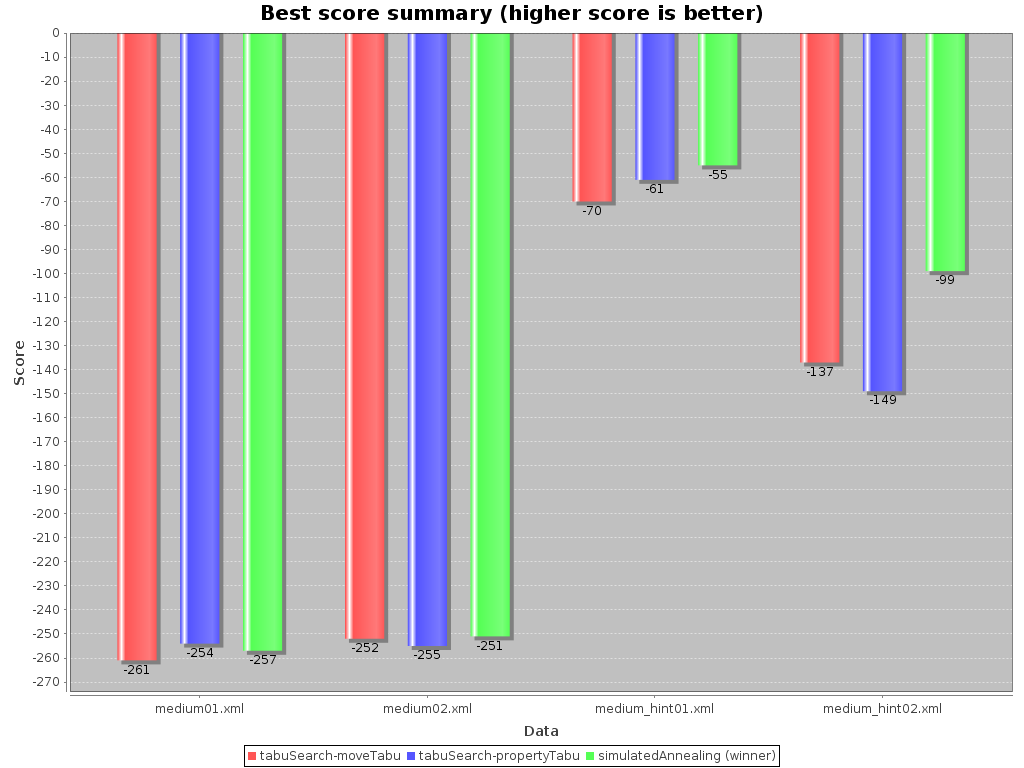
Shows the best score per problem scale for each solver configuration.
Useful for visualizing the scalability of each solver configuration.
Note
The problem scale will report 0 if any @ValueRangeProvider method
signature returns ValueRange (instead of CountableValueRange or
Collection).
Shows the winning score difference per inputSolutionFile for each solver configuration.
The winning score difference is the score difference with the score of the winning solver configuration for that
particular inputSolutionFile.
Useful for zooming in on the results of the best score summary.
Shows the return on investment (ROI) per inputSolutionFile for each solver configuration
if you'd upgrade from the worst solver configuration for that particular
inputSolutionFile.
Useful for visualizing the return on investment (ROI) to decision makers.
Shows the score calculation speed: the average calculation count per second per problem scale for each solver configuration.
Useful for comparing different score calculators and/or score rule implementations (presuming that the solver configurations do not differ otherwise). Also useful to measure the scalability cost of an extra constraint.
Shows the time spent per inputSolutionFile for each solver configuration. This is
pointless if it's benchmarking against a fixed time limit.
Useful for visualizing the performance of construction heuristics (presuming that no other solver phases are configured).
Shows the time spent per problem scale for each solver configuration. This is pointless if it's benchmarking against a fixed time limit.
Useful for extrapolating the scalability of construction heuristics (presuming that no other solver phases are configured).
Shows the best score per time spent for each solver configuration. This is pointless if it's benchmarking against a fixed time limit.
Useful for visualizing trade-off between the best score versus the time spent for construction heuristics (presuming that no other solver phases are configured).
The benchmarker supports outputting problem statistics as graphs and CSV (comma separated values) files to
the benchmarkDirectory. To configure one, add a problemStatisticType
line:
<plannerBenchmark>
<benchmarkDirectory>local/data/nqueens/solved</benchmarkDirectory>
<inheritedSolverBenchmark>
<problemBenchmarks>
...
<problemStatisticType>BEST_SCORE</problemStatisticType>
<problemStatisticType>CALCULATE_COUNT_PER_SECOND</problemStatisticType>
</problemBenchmarks>
...
</inheritedSolverBenchmark>
...
</plannerBenchmark>Multiple problemStatisticType elements are allowed.
Note
These statistic per dataset can slow down the solver noticeably, which affects the benchmark results. That's why they are optional and not enabled by default.
The non-optional summary statistics cannot slow down the solver noticeably.
The following types are supported:
To see how the best score evolves over time, add:
<problemBenchmarks>
...
<problemStatisticType>BEST_SCORE</problemStatisticType>
</problemBenchmarks>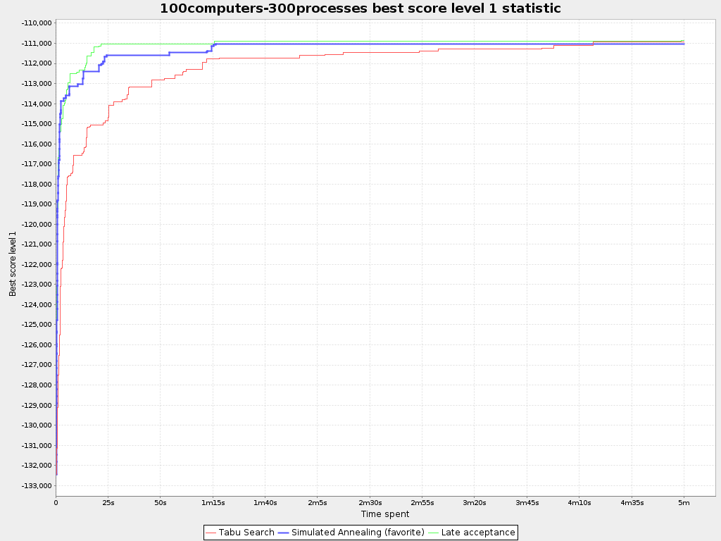
The best score over time statistic is very useful to detect abnormalities, such as a potential score trap.
Note
A time gradient based algorithm (such as Simulated Annealing) will have a different statistic if it's run with a different time limit configuration. That's because this Simulated Annealing implementation automatically determines its velocity based on the amount of time that can be spent. On the other hand, for the Tabu Search and Late Annealing, what you see is what you'd get.
To see how the step score evolves over time, add:
<problemBenchmarks>
...
<problemStatisticType>STEP_SCORE</problemStatisticType>
</problemBenchmarks>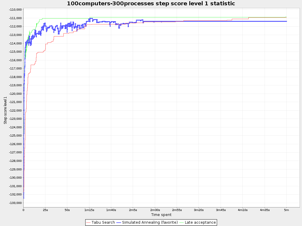
Compare the step score statistic with the best score statistic (especially on parts for which the best score flatlines). If it hits a local optima, the solver should take deteriorating steps to escape it. But it shouldn't deteriorate too much either.
Warning
The step score statistic has been seen to slow down the solver noticeably due to GC stress, especially for fast stepping algorithms (such as Simulated Annealing and Late Acceptance).
To see how fast the scores are calculated, add:
<problemBenchmarks>
...
<problemStatisticType>CALCULATE_COUNT_PER_SECOND</problemStatisticType>
</problemBenchmarks>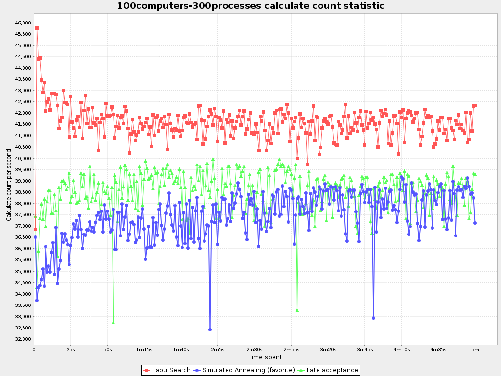
Note
The initial high calculate count is typical during solution initialization: it's far easier to calculate the score of a solution if only a handful planning entities have been initialized, than when all the planning entities are initialized.
After those few seconds of initialization, the calculate count is relatively stable, apart from an occasional stop-the-world garbage collector disruption.
To see how much each new best solution differs from the previous best solution, by counting the number of planning variables which have a different value (not including the variables that have changed multiple times but still end up with the same value), add:
<problemBenchmarks>
...
<problemStatisticType>BEST_SOLUTION_MUTATION</problemStatisticType>
</problemBenchmarks>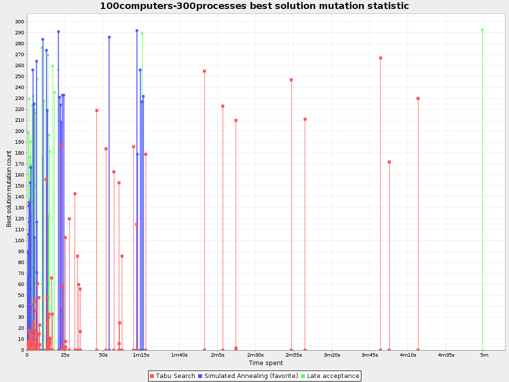
Use Tabu Search - an algorithm that behaves like a human - to get an estimation on how difficult it would be for a human to improve the previous best solution to that new best solution.
To see how the selected and accepted move count per step evolves over time, add:
<problemBenchmarks>
...
<problemStatisticType>MOVE_COUNT_PER_STEP</problemStatisticType>
</problemBenchmarks>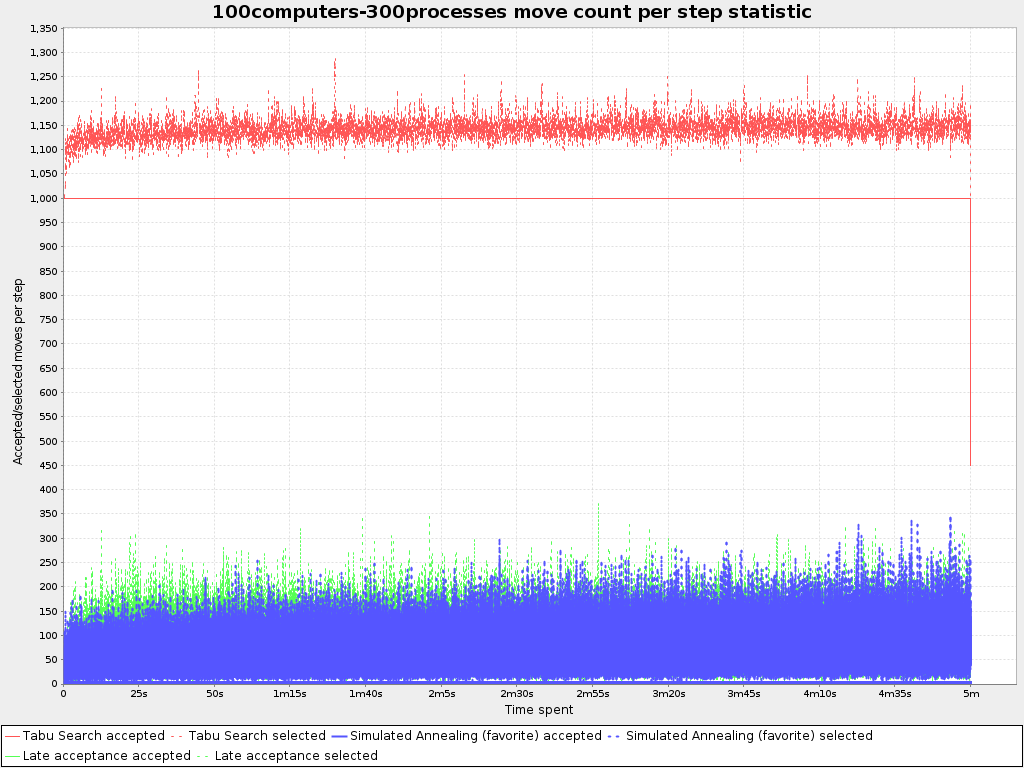
Warning
This statistic has been seen to slow down the solver noticeably due to GC stress, especially for fast stepping algorithms (such as Simulated Annealing and Late Acceptance).
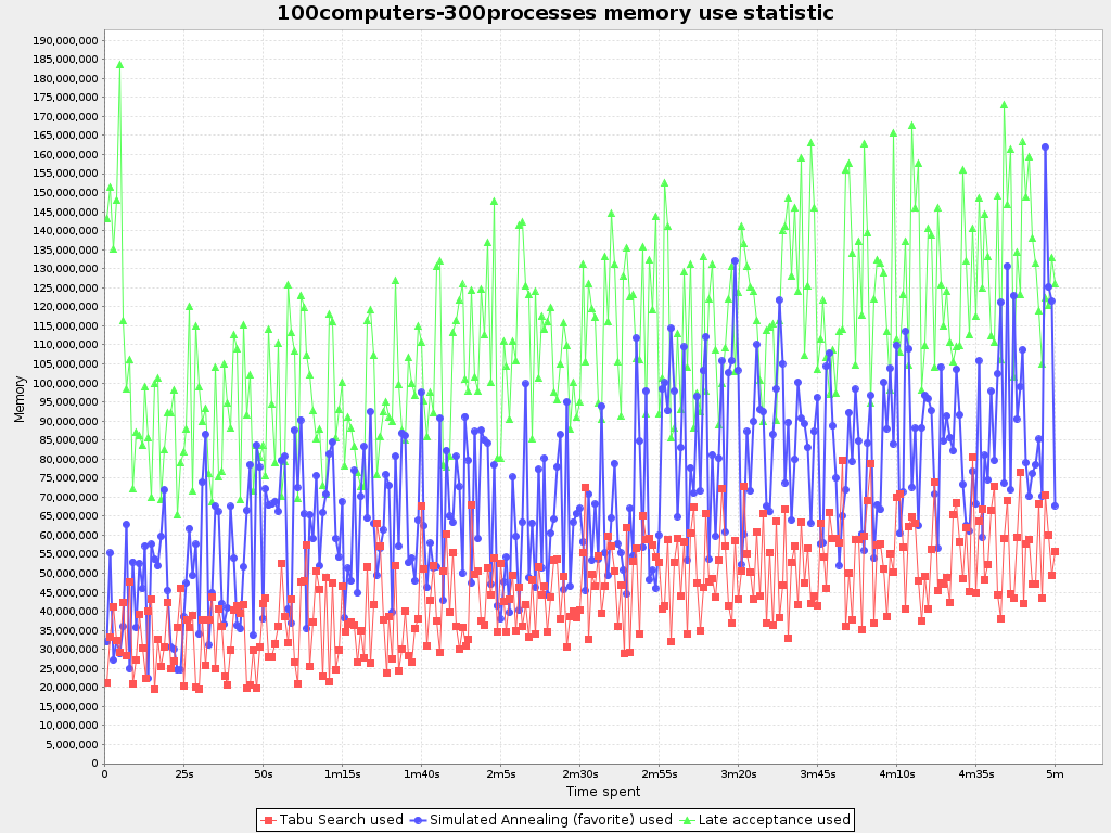
A single statistic is a statics for 1 dataset for 1 solver configuration. Unlike a problem statistic, it does not aggregate over solver configurations.
The benchmarker supports outputting single statistics as graphs and CSV (comma separated values) files to
the benchmarkDirectory. To configure one, add a singleStatisticType
line:
<plannerBenchmark>
<benchmarkDirectory>local/data/nqueens/solved</benchmarkDirectory>
<inheritedSolverBenchmark>
<problemBenchmarks>
...
<problemStatisticType>...</problemStatisticType>
<singleStatisticType>PICKED_MOVE_TYPE_BEST_SCORE_DIFF</singleStatisticType>
</problemBenchmarks>
...
</inheritedSolverBenchmark>
...
</plannerBenchmark>Multiple singleStatisticType elements are allowed.
Note
These statistic per single benchmark can slow down the solver noticeably, which affects the benchmark results. That's why they are optional and not enabled by default.
The following types are supported:
To see which constraints are matched in the best score (and how much) over time, add:
<problemBenchmarks>
...
<singleStatisticType>CONSTRAINT_MATCH_TOTAL_BEST_SCORE</singleStatisticType>
</problemBenchmarks>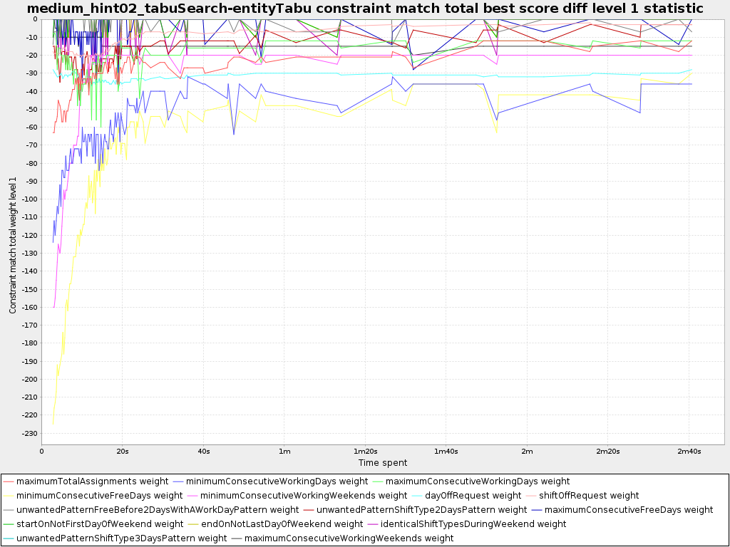
Requires the score calculation to support constraint matches. Drools score calculation supports constraint matches automatically, but incremental Java score calculation requires requires more work.
Warning
The constraint match total statistics has been seen to affect the solver noticeably.
To see which constraints are matched in the step score (and how much) over time, add:
<problemBenchmarks>
...
<singleStatisticType>CONSTRAINT_MATCH_TOTAL_STEP_SCORE</singleStatisticType>
</problemBenchmarks>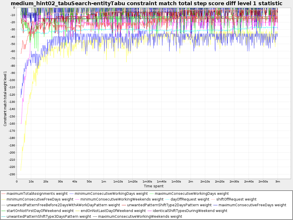
Requires the score calculation to support constraint matches. Drools score calculation supports constraint matches automatically, but incremental Java score calculation requires requires more work.
Warning
The constraint match total statistics has been seen to affect the solver noticeably.
To see which move types improve the best score (and how much) over time, add:
<problemBenchmarks>
...
<singleStatisticType>PICKED_MOVE_TYPE_BEST_SCORE_DIFF</singleStatisticType>
</problemBenchmarks>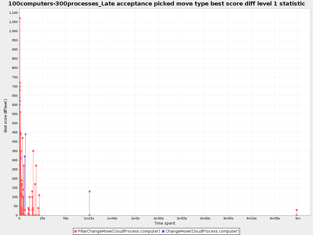
To see how much each winning step affects the step score over time, add:
<problemBenchmarks>
...
<singleStatisticType>PICKED_MOVE_TYPE_STEP_SCORE_DIFF</singleStatisticType>
</problemBenchmarks>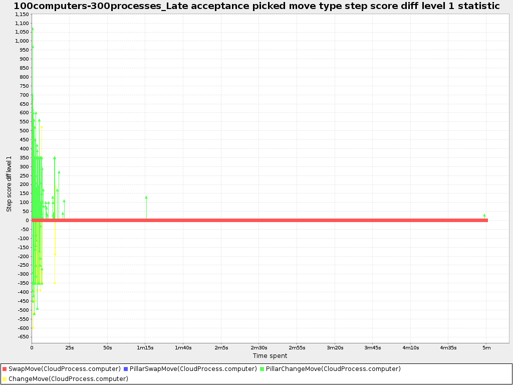
If you have multiple processors available on your computer, you can run multiple benchmarks in parallel on multiple threads to get your benchmarks results faster:
<plannerBenchmark>
...
<parallelBenchmarkCount>AUTO</parallelBenchmarkCount>
...
</plannerBenchmark>Warning
Running too many benchmarks in parallel will affect the results of benchmarks negatively. Leave some processors unused for garbage collection and other processes.
We tweak parallelBenchmarkCount AUTO to maximize the reliability
and efficiency of the benchmark results.
The following parallelBenchmarkCounts are supported:
1(default): Run all benchmarks sequentially.AUTO: Let Planner decide how many benchmarks to run in parallel. This formula is based on experience. It's recommended to prefer this over the other parallel enabling options.Static number: The number of benchmarks to run in parallel.
<parallelBenchmarkCount>2</parallelBenchmarkCount>JavaScript formula: Formula for the number of benchmarks to run in parallel. It can use the variable
availableProcessorCount. For example:<parallelBenchmarkCount>(availableProcessorCount / 2) + 1</parallelBenchmarkCount>
Note
The parallelBenchmarkCount is always limited to the number of available processors.
If it's higher, it will be automatically decreased.
Note
In the future, we will also support multi-JVM benchmarking. This feature is independent of multi-threaded solving or multi-JVM solving.
Matrix benchmarking is benchmarking a combination of value sets. For example: benchmark 4
entityTabuSize values (5, 7, 11 and
13) combined with 3 acceptedCountLimit values (500,
1000 and 2000), resulting in 12 solver configurations.
To reduce the verbosity of such a benchmark configuration, you can use a Freemarker template for the benchmark configuration instead:
<plannerBenchmark>
...
<inheritedSolverBenchmark>
...
</inheritedSolverBenchmark>
<#list [5, 7, 11, 13] as entityTabuSize>
<#list [500, 1000, 2000] as acceptedCountLimit>
<solverBenchmark>
<name>entityTabuSize ${entityTabuSize} acceptedCountLimit ${acceptedCountLimit}</name>
<solver>
<localSearch>
<unionMoveSelector>
<changeMoveSelector/>
<swapMoveSelector/>
</unionMoveSelector>
<acceptor>
<entityTabuSize>${entityTabuSize}</entityTabuSize>
</acceptor>
<forager>
<acceptedCountLimit>${acceptedCountLimit}</acceptedCountLimit>
</forager>
</localSearch>
</solver>
</solverBenchmark>
</#list>
</#list>
</plannerBenchmark>And build it with the class PlannerBenchmarkFactory:
PlannerBenchmarkFactory plannerBenchmarkFactory = PlannerBenchmarkFactory.createFromFreemarkerXmlResource(
"org/optaplanner/examples/cloudbalancing/benchmark/cloudBalancingBenchmarkConfigTemplate.xml.ftl");
PlannerBenchmark plannerBenchmark = benchmarkFactory.buildPlannerBenchmark();The BenchmarkAggregator takes 1 or more existing benchmarks and merges them into new
benchmark report, without actually running the benchmarks again.
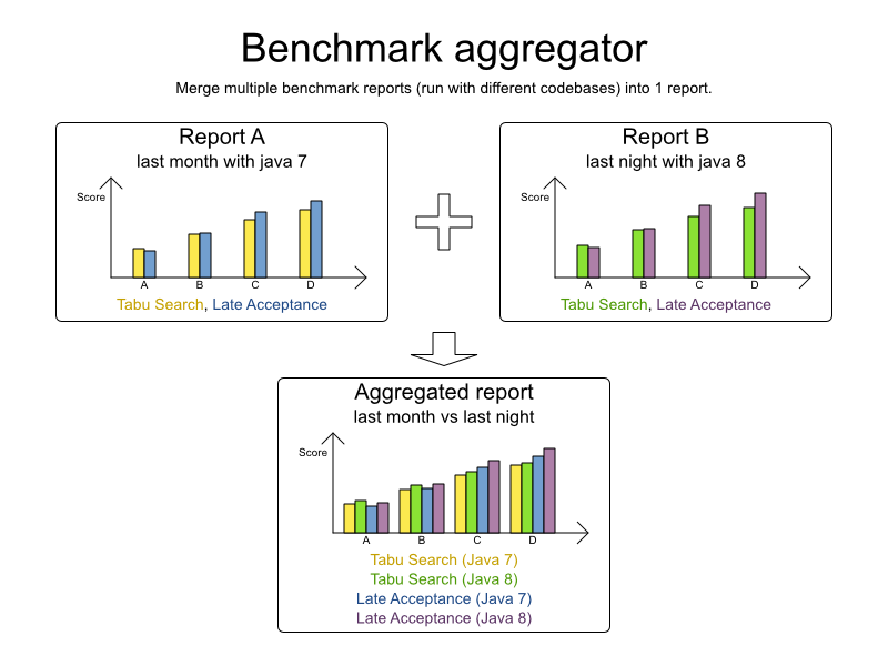
This is useful to:
Report on the impact of code changes: Run the same benchmark configuration before and after the code changes, then aggregate a report.
Report on the impact of dependency upgrades: Run the same benchmark configuration before and after upgrading the dependency, then aggregate a report.
Condense a too verbose report: Select only the interesting solver benchmarks from the existing report. This especially useful on template reports to make the graphs readable.
Partially rerun a benchmark: Rerun part of an existing report (for example only the failed or invalid solvers), then recreate the original intended report with the new values.
To use it, provide a PlannerBenchmarkFactory to the
BenchmarkAggregatorFrame to display the GUI:
public static void main(String[] args) {
PlannerBenchmarkFactory plannerBenchmarkFactory = PlannerBenchmarkFactory.createFromXmlResource(
"org/optaplanner/examples/nqueens/benchmark/nqueensBenchmarkConfig.xml");
BenchmarkAggregatorFrame.createAndDisplay(plannerBenchmarkFactory);
}Warning
Despite that it uses a benchmark configuration as input, it ignores all elements of that configuration,
except for the elements <benchmarkDirectory> and
<benchmarkReport>.
In the GUI, select the interesting benchmarks and click the button to generate the report.
The world constantly changes. The problem facts used to create a solution, might change before or during the execution of that solution. There are different situations (which can be combined):
Unforeseen fact changes: For example: an employee assigned to a shift calls in sick, an airplane scheduled to take off has a technical delay, one of the machines or vehicles break down, ... Use backup planning.
Impossible to assign all entities now: Leave some unassigned. For example: there are 10 shifts at the same time to assign but only 9 employees to handle shifts. Use overconstrained planning.
Unknown long term future facts: For example: The hospital admissions for the next 2 weeks are reliable, but those for week 3 and 4 are less reliable and for week 5 and beyond are not worth planning yet. Use continuous planning.
Constantly changing problem facts: Use real-time planning.
Waiting to start planning - to lower the risk of problem facts changing - usually isn't a good way to deal with that. More CPU time means a better planning solution. An incomplete plan is better than no plan.
Luckily, the optimization algorithms support planning a solution that's already (partially) planned, known as repeated planning.
Backup planning is the technique of adding extra score constraints to create space in the planning for when things go wrong. That creates a backup plan in the plan. For example: try to assign an employee as the spare employee (1 for every 10 shifts at the same time), keep 1 hospital bed open in each department, ...
Then, when things go wrong (one of the employees calls in sick), change the problem facts on the original solution (delete the sick employee leave his/her shifts unassigned) and just restart the planning, starting from that solution, which has a different score now. The construction heuristics will fill in the newly created gaps (probably with the spare employee) and the metaheuristics will even improve it further.
When there is no feasible solution to assign all planning entities, it's often desired to assign as many entities as possible without breaking hard constraints. This is called overconstrained planning.
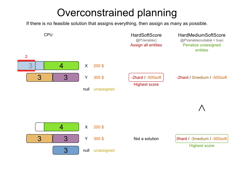
To implement this:
Add a additional score level (usually a medium level between the hard and soft level) by switching ScoreDefinition.
Make the planning variable nullable.
Add a score constraint on the new level (so usually a medium constraint) to penalize the number of unassigned entities (or a weighted sum of them).
Continuous planning is the technique of planning one or more upcoming planning windows at the same time and repeating that process monthly, weekly, daily or hourly. Because time is infinite, there are infinite future windows, so planning all future windows is impossible. Instead, plan only a fixed number of upcoming planning windows.
Past planning windows are immutable. The first upcoming planning window is considered stable (unlikely to change), while later upcoming planning windows are considered draft (likely to change during the next planning effort). Distant future planning windows are not planned at all.
Past planning windows have only immovable planning entities: the planning entities can no longer be changed (they are unable to move), but some of them are still needed in the score calculation, as they might affect some of the score constraints that apply on the upcoming planning entities. For example: when an employee should not work more than 5 days in a row, he shouldn't work today and tomorrow if he worked the past 4 days already.
Sometimes some planning entities are semi-immovable: they can be changed, but occur a certain score penalty if they differ from their original place. For example: avoid rescheduling hospital beds less than 2 days before the patient arrives (unless it's really worth it), avoid changing the airplane gate during the 2 hours before boarding (unless there is no alternative), ...
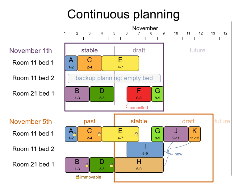
Notice the difference between the original planning of November 1th and the new planning of November 5th: some problem facts (F, H, I, J, K) changed, which results in unrelated planning entities (G) changing too.
To make some planning entities immovable, simply add an entity SelectionFilter that
returns true if an entity is movable and false if it is immovable.
public class MovableShiftAssignmentSelectionFilter implements SelectionFilter<ShiftAssignment> {
public boolean accept(ScoreDirector scoreDirector, ShiftAssignment shiftAssignment) {
ShiftDate shiftDate = shiftAssignment.getShift().getShiftDate();
NurseRoster nurseRoster = (NurseRoster) scoreDirector.getWorkingSolution();
return nurseRoster.getNurseRosterInfo().isInPlanningWindow(shiftDate);
}
}And configure it like this:
@PlanningEntity(movableEntitySelectionFilter = MovableShiftAssignmentSelectionFilter.class)
public class ShiftAssignment {
...
}Warning
Custom MoveListFactory and MoveIteratorFactory implementations must
make sure that they don't move immovable entities.
Replanning an existing plan can be very disruptive on the plan. If the plan affects humans (such as employees, drivers, ...), very disruptive changes are often undesirable. In such cases, nonvolatile replanning helps: the gain of changing a plan must be higher than the disruption it causes.
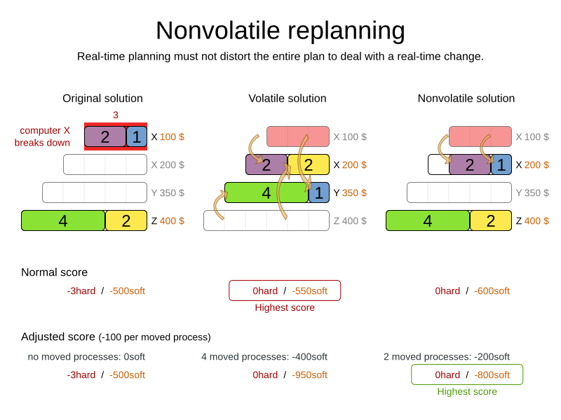
For example, in the Machine Reassignment example, the entity has both the planning variable
machine and its original value originalMachine:
@PlanningEntity(...)
public class ProcessAssignment {
private MrProcess process;
private Machine originalMachine;
private Machine machine;
public Machine getOriginalMachine() {...}
@PlanningVariable(...)
public Machine getMachine() {...}
public boolean isMoved() {
return originalMachine != null && originalMachine != machine;
}
...
}During planning, the planning variable machine changes. By comparing it with the
originalMachine, a change in plan can be penalized:
rule "processMoved"
when
ProcessAssignment(moved == true)
then
scoreHolder.addSoftConstraintMatch(kcontext, -1000);
endThe soft penalty of -1000 means that a better solution is only accepted if it improves
the soft score for at least 1000 points per variable changed (or if it improves the hard
score).
To do real-time planning, first combine backup planning and continuous planning with short planning windows to lower the burden of real-time planning. As time passes, the problem itself changes:
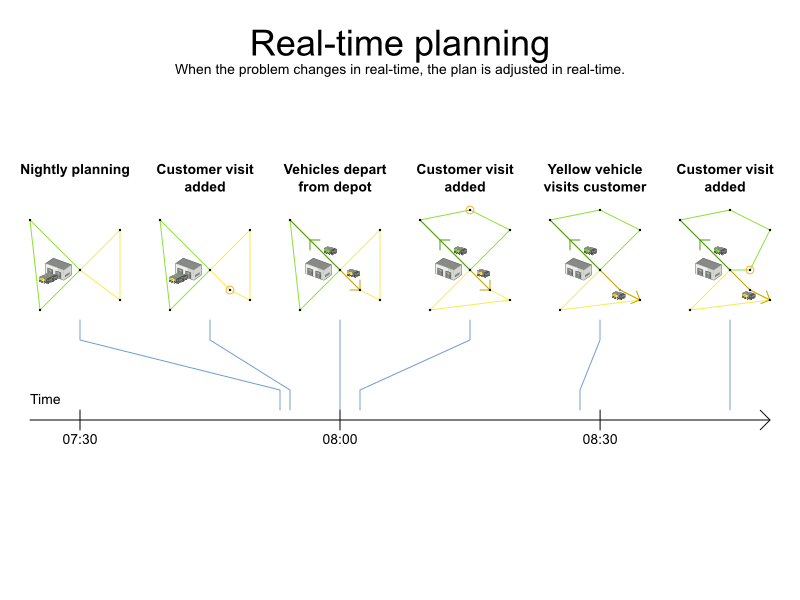
In the example above, 3 customers are added at different times (07:56,
08:02 and 08:45), after the original customer set finished solving at
07:55 and in some cases after the vehicles already left. Planner can handle such scenario's with
ProblemFactChange (in combination with immovable
planning entities).
While the Solver is solving, an outside event might want to change one of the problem
facts, for example an airplane is delayed and needs the runway at a later time. Do not change the problem fact
instances used by the Solver while it is solving (from another thread or even in the same
thread), as that will corrupt it. Instead, add a ProblemFactChange to the
Solver which it will execute in the solver thread as soon as possible.
public interface Solver {
...
boolean addProblemFactChange(ProblemFactChange problemFactChange);
boolean isEveryProblemFactChangeProcessed();
...
}public interface ProblemFactChange {
void doChange(ScoreDirector scoreDirector);
}Here's an example:
public void deleteComputer(final CloudComputer computer) {
solver.addProblemFactChange(new ProblemFactChange() {
public void doChange(ScoreDirector scoreDirector) {
CloudBalance cloudBalance = (CloudBalance) scoreDirector.getWorkingSolution();
// First remove the problem fact from all planning entities that use it
for (CloudProcess process : cloudBalance.getProcessList()) {
if (ObjectUtils.equals(process.getComputer(), computer)) {
scoreDirector.beforeVariableChanged(process, "computer");
process.setComputer(null);
scoreDirector.afterVariableChanged(process, "computer");
}
}
// A SolutionCloner does not clone problem fact lists (such as computerList)
// Shallow clone the computerList so only workingSolution is affected, not bestSolution or guiSolution
cloudBalance.setComputerList(new ArrayList<CloudComputer>(cloudBalance.getComputerList()));
// Next remove it the problem fact itself
for (Iterator<CloudComputer> it = cloudBalance.getComputerList().iterator(); it.hasNext(); ) {
CloudComputer workingComputer = it.next();
if (ObjectUtils.equals(workingComputer, computer)) {
scoreDirector.beforeProblemFactRemoved(workingComputer);
it.remove(); // remove from list
scoreDirector.beforeProblemFactRemoved(workingComputer);
break;
}
}
}
});
}Warning
Any change on the problem facts or planning entities in a ProblemFactChange must be
told to the ScoreDirector.
Important
To write a ProblemFactChange correctly, it's important to understand the behaviour of
a planning clone:
Any change in a
ProblemFactChangemust be done on theSolutioninstance ofscoreDirector.getWorkingSolution(). TheworkingSolutionis a planning clone of theBestSolutionChangedEvent'sbestSolution. So theworkingSolutionin theSolveris never the same instance as theSolutionin the rest of your application.A planning clone also clones the planning entities and planning entity collections. So any change on the planning entities must happen on the instances hold by
scoreDirector.getWorkingSolution().A planning clone does not clone the problem facts, nor the problem fact collections. Therefore the
workingSolutionand thebestSolutionshare the same problem fact instances and the same problem fact list instances.Any problem fact or problem fact list changed by a
ProblemFactChangemust be problem cloned first (which can imply rerouting references in other problem facts and planning entities). Otherwise, if theworkingSolutionandbestSolutionare used in different threads (for example a solver thread and a GUI event thread), a race condition can occur.
Note
Many types of changes can leave a planning entity uninitialized, resulting in a partially initialized solution. That's fine, as long as the first solver phase can handle it. All construction heuristics solver phases can handle that, so it's recommended to configure such a solver phase as the first phase.
In essence, the Solver stops, runs the ProblemFactChange and restarts. This is a warm start because its initial solution is the
adjusted best solution of the previous run. Each solver phase runs again. This implies the construction heuristic
runs again, but because little or no planning variables are uninitialized (unless you have a nullable planning variable), it finishes much quicker than in a cold
start.
Each configured Termination resets (both in solver and phase configuration), but a
previous call to terminateEarly() is not undone. Normally however, you won't configure any
Termination (except in daemon mode), just call Solver.terminateEarly() when
the results are needed. Alternatively, do configure a Termination and use the daemon mode in
combination with BestSolutionChangedEvent as
described below.
In real-time planning, it's often useful to have a solver thread wait when it runs out of work, and
immediately resume solving a problem once new problem fact changes are added. Putting the
Solver in daemon mode has these effects:
If the
Solver'sTerminationterminates, it does not return fromsolve()but blocks its thread instead (which frees up CPU power).Except for terminateEarly(), which does make it return from
solve(), freeing up system resources and allowing an application to shutdown gracefully.If a
Solverstarts with an empty planning entity collection, it waits in the blocked state immediately.
If a
ProblemFactChangeis added, it goes into the running state, applies theProblemFactChangeand runs theSolveragain.
To configure the daemon mode:
<solver>
<daemon>true</daemon>
...
</solver>Warning
Don't forget to call Solver.terminateEarly() when your application needs to shutdown to
avoid killing the solver thread unnaturally.
Subscribe to the BestSolutionChangedEvent to
process new best solutions found by the solver thread. A BestSolutionChangedEvent doesn't
guarantee that every ProblemFactChange has been processed already, nor that the solution is
initialized and feasible. To ignore BestSolutionChangedEvents with such invalid solutions, do
this:
public void bestSolutionChanged(BestSolutionChangedEvent<CloudBalance> event) {
// Ignore invalid solutions
if (event.isEveryProblemFactChangeProcessed()
&& event.isNewBestSolutionInitialized()
&& event.getNewBestSolution().getScore().isFeasible()) {
...
}
}Planner's input and output data (the planning problem and the best solution) are plain old JavaBeans (POJO's), so integration with other Java technologies is straightforward. For example:
To read a planning problem from the database (and store the best solution in it), annotate the domain POJO's with JPA annotations.
To read a planning problem from an XML file (and store the best solution in it), annotate the domain POJO's with XStream or JAXB annotations.
To expose the Solver as a REST Service that reads the planning problem and responds with the best solution, annotate the domain POJO's with XStream or JAXB annotations and hook the
Solverin Camel or RESTEasy.
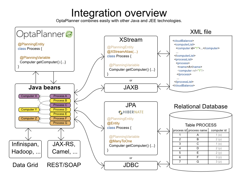
Enrich the domain POJO's (solution, entities and problem facts) with JPA annotations to store them in a database.
Note
Do not confuse JPA's @Entity annotation with Planner's
@PlanningEntity annotation. They can appear both on the same class.
Enrich the domain POJO's (solution, entities and problem facts) with XStream annotations to serialize them to/from XML.
Camel is an enterprise integration framework which includes support for Planner (starting from Camel 2.13). It can expose a use case as a REST service, a SOAP service, a JMS service, ...
Read the documentation for the camel-optaplanner component. That component works in Karaf too.
To deploy an Planner web application on WildFly, simply include the optaplanner dependency jars in the
war file's WEB-INF/lib directory (just like any other dependency) as shown
in the optaplanner-webexamples-*.war. However, in this approach the war file can easily grow to
several MB in size, which is fine for a one-time deployment, but too heavyweight for frequent redeployments
(especially over a slow network connection).
The remedy is to use deliver the optaplanner jars in a JBoss module to WildFly and create a skinny war. Let's create an module called org.optaplanner:
Navigate to the directory
${WILDFLY_HOME}/modules/system/layers/base/. This directory contains the JBoss modules of WildFly. Create directory structureorg/optaplanner/mainfor our new module.Copy
optaplanner-core-${version}.jarand all its direct and transitive dependency jars into that new directory. Use "mvn dependency:tree" on each optaplanner artifact to discover all dependencies.Create the file
module.xmlin that new directory. Give it this content:<?xml version="1.0" encoding="UTF-8"?> <module xmlns="urn:jboss:module:1.3" name="org.optaplanner"> <resources> ... <resource-root path="kie-api-${version}.jar"/> ... <resource-root path="optaplanner-core-${version}.jar"/> ... <resource-root path="."/> </resources> <dependencies> <module name="javaee.api"/> </dependencies> </module>
Navigate to the deployed
warfile.Remove
optaplanner-core-${version}.jarand all its direct and transitive dependency jars from theWEB-INF/libdirectory in thewarfile.Create the file
jboss-deployment-structure.xmlin theWEB-INF/libdirectory. Give it this content:<?xml version="1.0" encoding="UTF-8" ?> <jboss-deployment-structure> <deployment> <dependencies> <module name="org.optaplanner" export="true"/> </dependencies> </deployment> </jboss-deployment-structure>
Important
Because of WildFly's class loading, the method SolverFactory.createFromXmlResource()
might not find the solver configuration and throw an IllegalArgumentException. Instead
use:
SolverFactory solverFactory = SolverFactory.createFromXmlInputStream(
getClass().getClassLoader().getResourceAsStream(
"org/optaplanner/examples/nqueens/solver/nqueensSolverConfig.xml"));The optaplanner-core jar includes OSGi metadata in its MANIFEST.MF
file to function properly in an OSGi environment too.
Furthermore, the maven artifact drools-karaf-features (which will be renamed to
kie-karaf-features) contains a features.xml file that supports the
OSGi-feature optaplanner-engine.
Note
Planner does not require OSGi. It works perfectly fine in a normal Java environment too.
Android is not a complete JVM (because some JDK libraries are missing), but Planner works on Android with easy Java or incremental Java score calculation. The Drools rule engine does not work on Android yet, so Drools score calculation doesn't work on Android and its dependencies need to be excluded.
Workaround to use Planner on Android:
Add a dependency to the
build.gradlefile in your Android project to excludeorg.droolsandxmlpulldependencies:dependencies { ... compile('org.optaplanner:optaplanner-core:...') { exclude group: 'xmlpull' exclude group: 'org.drools' } ... }
A good Planner implementation beats any good human planner for non-trivial datasets. Many human planners fail to accept this, often because they feel threatened by an automated system.
But despite that, both can benefit if the human planner acts as supervisor to Planner:
The human planner defines and validates the score function.
Some examples expose a
*Parametrizationobject, which defines the weight for each score constraint. The human planner can then tweak those weights at runtime.When the business changes, the score function often needs to change too. The human planner can notify the developers to add, change or remove score constraints.
The human planner is always in control of Planner.
As shown in the course scheduling example, the human planner can lock 1 or more planning variables to a specific planning value and make those immovable. Because they are immovable, Planner does not change them: it optimizes the planning around the enforcements made by the human. If the human planner locks all planning variables, he/she sidelines Planner completely.
In a prototype implementation, the human planner might use this occasionally. But as the implementation matures, it must become obsolete. But do keep the feature alive: as a reassurance for the humans. Or in case that one day the business changes dramatically before the score constraints can be adjusted.
Therefore, it's often a good idea to involve the human planner in your project.
The diagram below explains the overall structure of the OptaPlanner source code:
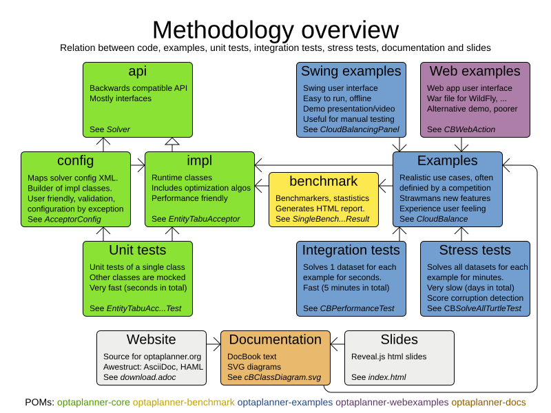
The development philosophy includes:
Reuse: The examples are reused as integration tests, stress tests and demo's. The documentation images are reused as slides.
Consistent terminology: Each example has a class
App(executable class),Dao(Data Access Object) andPanel(swing UI).Consistent structure: Each example has the same packages:
domain,persistence,app,solverandswingui.Real world usefulness: Every feature is used in an example. Most examples are real world use cases with real world constraints, often with real world data.
Automated testing: There are unit tests, integration tests and stress tests. The test coverage is high.
Fail fast with an understandable error message: Invalid states are checked as early as possible.
Fail fast. There are several levels of fail fast, from better to worse:
Fail Fast at compile time. For example: Don't accept an
Objectas parameter if it needs to be aStringor anInteger.Fail Fast at startup time. For example: if the configuration parameter needs to be a positive
intand it's negative, fail fastFail Fast at runtime. For example: if the request needs to contain a double between
0.0and1.0and it's bigger than1.0, fail fast.Fail Fast at runtime in assertion mode if the detection performance cost is high. For example: If, after every low level iteration, the variable A needs to be equal to the square root of B, check it if and only if an assert flag is set to true (usually controlled by the EnvironmentMode).
ExceptionmessagesThe
Exceptionmessage must include the name and state of each relevant variable. For example:if (fooSize < 0) { throw new IllegalArgumentException("The fooSize (" + fooSize + ") of bar (" + this + ") must be positive."); }Notice that the output clearly explains what's wrong:
Exception in thread "main" java.lang.IllegalArgumentException: The fooSize (-5) must be positive. at ...Whenever possible, the
Exceptionmessage must include context.Whenever the fix is not obvious, the
Exceptionmessage must include advice.Exception in thread "main" java.lang.IllegalArgumentException: UndoMove corruption: ... 1) Check your custom createUndoMove() of ... 2) Check your custom Variable listeners if ... at ...