
1. OptaPlanner introduction
1.1. What is OptaPlanner?
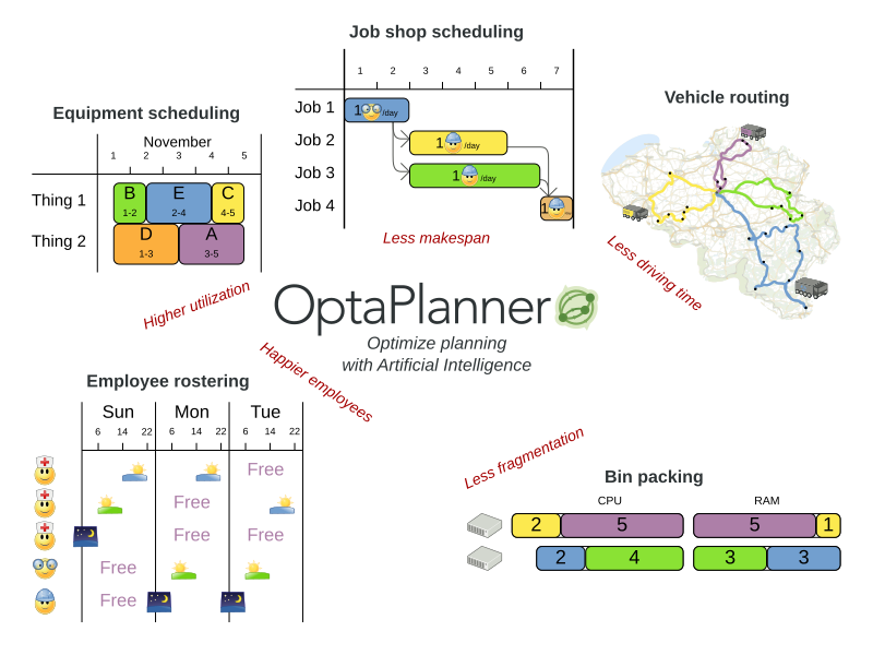
Every organization faces planning problems: providing products or services with a limited set of constrained resources (employees, assets, time and money). OptaPlanner optimizes such planning to do more business with less resources. This is known as Constraint Satisfaction Programming (which is part of the Operations Research discipline).
OptaPlanner is a lightweight, embeddable constraint satisfaction engine which optimizes planning problems. It solves use cases such as:
-
Employee shift rostering: timetabling nurses, repairmen, …
-
Agenda scheduling: scheduling meetings, appointments, maintenance jobs, advertisements, …
-
Educational timetabling: scheduling lessons, courses, exams, conference presentations, …
-
Vehicle routing: planning vehicle routes (trucks, trains, boats, airplanes, …) for moving freight and/or passengers through multiple destinations using known mapping tools …
-
Bin packing: filling containers, trucks, ships, and storage warehouses with items, but also packing information across computer resources, as in cloud computing …
-
Job shop scheduling: planning car assembly lines, machine queue planning, workforce task planning, …
-
Cutting stock: minimizing waste while cutting paper, steel, carpet, …
-
Sport scheduling: planning games and training schedules for football leagues, baseball leagues, …
-
Financial optimization: investment portfolio optimization, risk spreading, …
1.2. What is a planning problem?
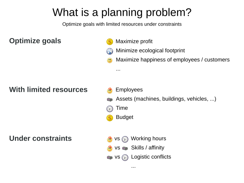
A planning problem has an optimal goal, based on limited resources and under specific constraints. Optimal goals can be any number of things, such as:
-
Maximized profits - the optimal goal results in the highest possible profit.
-
Minimized ecological footprint - the optimal goal has the least amount of environmental impact.
-
Maximized satisfaction for employees or customers - the optimal goal prioritizes the needs of employees or customers.
The ability to achieve these goals relies on the number of resources available, such as:
-
The number of people.
-
Amount of time.
-
Budget.
-
Physical assets, for example, machinery, vehicles, computers, buildings, etc.
Specific constraints related to these resources must also be taken into account, such as the number of hours a person works, their ability to use certain machines, or compatibility between pieces of equipment.
OptaPlanner helps JavaTM programmers solve constraint satisfaction problems efficiently. Under the hood, it combines optimization heuristics and metaheuristics with very efficient score calculation.
1.2.1. A planning problem is NP-complete or NP-hard
All the use cases above are probably NP-complete/NP-hard, which means in layman’s terms:
-
It’s easy to verify a given solution to a problem in reasonable time.
-
There is no silver bullet to find the optimal solution of a problem in reasonable time (*).
|
(*) At least, none of the smartest computer scientists in the world have found such a silver bullet yet. But if they find one for 1 NP-complete problem, it will work for every NP-complete problem. In fact, there’s a $ 1,000,000 reward for anyone that proves if such a silver bullet actually exists or not. |
The implication of this is pretty dire: solving your problem is probably harder than you anticipated, because the two common techniques won’t suffice:
-
A Brute Force algorithm (even a smarter variant) will take too long.
-
A quick algorithm, for example in bin packing, putting in the largest items first, will return a solution that is far from optimal.
By using advanced optimization algorithms, OptaPlanner does find a near-optimal solution in reasonable time for such planning problems.
1.2.2. A planning problem has (hard and soft) constraints
Usually, a planning problem has at least two levels of constraints:
-
A (negative) hard constraint must not be broken. For example: 1 teacher cannot teach 2 different lessons at the same time.
-
A (negative) soft constraint should not be broken if it can be avoided. For example: Teacher A does not like to teach on Friday afternoon.
Some problems have positive constraints too:
-
A positive soft constraint (or reward) should be fulfilled if possible. For example: Teacher B likes to teach on Monday morning.
Some basic problems (such as N queens) only have hard constraints. Some problems have three or more levels of constraints, for example hard, medium and soft constraints.
These constraints define the score calculation (AKA fitness function) of a planning problem. Each solution of a planning problem can be graded with a score. With OptaPlanner, score constraints are written in an Object Oriented language, such as JavaTM code. Such code is easy, flexible and scalable.
1.2.3. A planning problem has a huge search space
A planning problem has a number of solutions. There are several categories of solutions:
-
A possible solution is any solution, whether or not it breaks any number of constraints. Planning problems tend to have an incredibly large number of possible solutions. Many of those solutions are worthless.
-
A feasible solution is a solution that does not break any (negative) hard constraints. The number of feasible solutions tends to be relative to the number of possible solutions. Sometimes there are no feasible solutions. Every feasible solution is a possible solution.
-
An optimal solution is a solution with the highest score. Planning problems tend to have 1 or a few optimal solutions. There is always at least 1 optimal solution, even in the case that there are no feasible solutions and the optimal solution isn’t feasible.
-
The best solution found is the solution with the highest score found by an implementation in a given amount of time. The best solution found is likely to be feasible and, given enough time, it’s an optimal solution.
Counterintuitively, the number of possible solutions is huge (if calculated correctly), even with a small dataset. As you can see in the examples, most instances have a lot more possible solutions than the minimal number of atoms in the known universe (10^80). Because there is no silver bullet to find the optimal solution, any implementation is forced to evaluate at least a subset of all those possible solutions.
OptaPlanner supports several optimization algorithms to efficiently wade through that incredibly large number of possible solutions. Depending on the use case, some optimization algorithms perform better than others, but it’s impossible to tell in advance. With OptaPlanner, it is easy to switch the optimization algorithm, by changing the solver configuration in a few lines of XML or code.
1.3. Requirements
OptaPlanner is open source software, released under the Apache License 2.0. This license is very liberal and allows reuse for commercial purposes. Read the layman’s explanation.
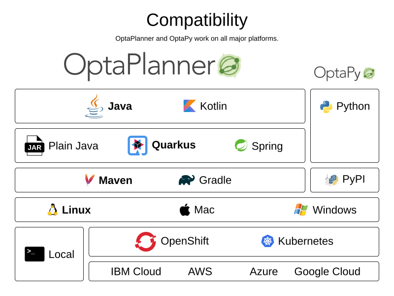
OptaPlanner is 100% pure JavaTM and runs on Java 11 or higher. It integrates very easily with other JavaTM technologies. OptaPlanner is available in the Maven Central Repository.
OptaPlanner works on any Java Virtual Machine and is compatible with the major JVM languages and all major platforms.
1.4. Governance
1.4.1. Status of OptaPlanner
OptaPlanner is stable, reliable and scalable. It has been heavily tested with unit, integration, and stress tests, and is used in production throughout the world. One example handles over 50 000 variables with 5000 values each, multiple constraint types and billions of possible constraint matches.
See Release notes for an overview of recent activity in the project.
1.4.2. Backwards compatibility
OptaPlanner separates its API and implementation:
-
Public API: All classes in the package namespace org.optaplanner.core.api, org.optaplanner.benchmark.api, org.optaplanner.test.api and org.optaplanner.persistence…api are 100% backwards compatible in future releases (especially minor and hotfix releases). In rare circumstances, if the major version number changes, a few specific classes might have a few backwards incompatible changes, but those will be clearly documented in the upgrade recipe.
-
XML configuration: The XML solver configuration is backwards compatible for all elements, except for elements that require the use of non-public API classes. The XML solver configuration is defined by the classes in the package namespace org.optaplanner.core.config and org.optaplanner.benchmark.config.
-
Implementation classes: All other classes are not backwards compatible. They will change in future major or minor releases (but probably not in hotfix releases). The upgrade recipe describes every such relevant change and on how to quickly deal with it when upgrading to a newer version.
|
This documentation covers some |
1.4.3. Community and support
For news and articles, check our blog,
twitter (including Geoffrey’s twitter)
and facebook.
If you’re happy with OptaPlanner, make us happy by posting a tweet or blog article about it.
Public questions are welcome on here. Bugs and feature requests are welcome in our issue tracker. Pull requests are very welcome on GitHub and get priority treatment! By open sourcing your improvements, you’ll benefit from our peer review and from our improvements made on top of your improvements.
Red Hat sponsors OptaPlanner development by employing the core team. For enterprise support and consulting, take a look at these services.
1.4.4. Relationship with KIE
OptaPlanner is part of the KIE group of projects. It releases regularly (typically every 3 weeks) together.
See the architecture overview to learn more about the optional integration with Drools.
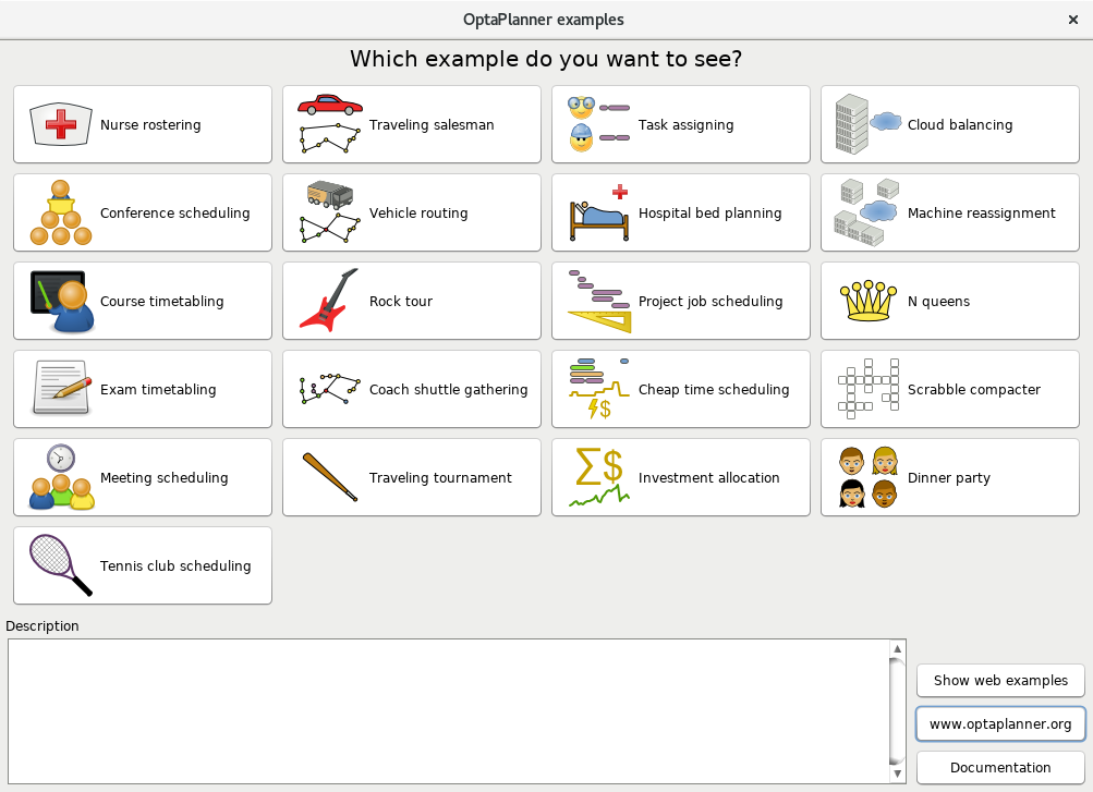
1.5. Download and run the examples
1.5.1. Get the release ZIP and run the examples
To try it now:
-
Download a release zip of OptaPlanner from the OptaPlanner website and unzip it.
-
Open the directory examples and run the script.
Linux or Mac:
$ cd examples
$ ./runExamples.sh
Windows:
$ cd examples
$ runExamples.bat
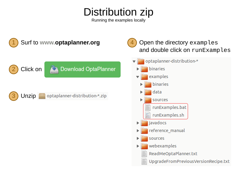
The Examples GUI application will open. Pick an example to try it out:
|
OptaPlanner itself has no GUI dependencies. It runs just as well on a server or a mobile JVM as it does on the desktop. |
1.5.2. Run the examples in an IDE
To run the examples in IntelliJ IDEA, VSCode or Eclipse:
-
Open the file examples/sources/pom.xml as a new project, the maven integration will take care of the rest.
-
Run the examples from the project.
1.5.3. Use OptaPlanner with Maven, Gradle, or ANT
The OptaPlanner jars are available in the central maven repository (and the snapshots in the JBoss maven repository).
If you use Maven, add a dependency to optaplanner-core in your pom.xml:
    <dependency>
      <groupId>org.optaplanner</groupId>
      <artifactId>optaplanner-core</artifactId>
      <version>...</version>
    </dependency>
Or better yet, import the optaplanner-bom in dependencyManagement to avoid duplicating version numbers
when adding other optaplanner dependencies later on:
<project>
  ...
  <dependencyManagement>
    <dependencies>
      <dependency>
        <groupId>org.optaplanner</groupId>
        <artifactId>optaplanner-bom</artifactId>
        <type>pom</type>
        <version>...</version>
        <scope>import</scope>
      </dependency>
    </dependencies>
  </dependencyManagement>
  <dependencies>
    <dependency>
      <groupId>org.optaplanner</groupId>
      <artifactId>optaplanner-core</artifactId>
    </dependency>
    <dependency>
      <groupId>org.optaplanner</groupId>
      <artifactId>optaplanner-persistence-jpa</artifactId>
    </dependency>
    ...
  </dependencies>
</project>
If you use Gradle, add a dependency to optaplanner-core in your build.gradle:
dependencies {
  implementation 'org.optaplanner:optaplanner-core:...'
}
If you’re still using ANT, copy all the jars from the download zip’s binaries directory in your classpath.
|
The download zip’s Check the maven repository |
1.5.4. Build OptaPlanner from source
Prerequisites
Build and run the examples from source.
-
Clone
optaplannerfrom GitHub (or alternatively, download the zipball):$ git clone https://github.com/kiegroup/optaplanner.git ... -
Build it with Maven:
$ cd optaplanner
$ mvn clean install -DskipTests
...
The first time, Maven might take a long time, because it needs to download jars.
-
Run the examples:
$ cd optaplanner-examples $ mvn exec:java ... -
Edit the sources in your favorite IDE.
2. Quick start
2.1. Overview
Each quick start gets you up and running with OptaPlanner quickly. Pick the quick start that best aligns with your requirements:
-
-
Build a simple Java application that uses OptaPlanner to optimize a school timetable for students and teachers.
-
-
Quarkus Java (recommended)
-
Build a REST application that uses OptaPlanner to optimize a school timetable for students and teachers.
-
Quarkus is an extremely fast platform in the Java ecosystem. It is ideal for rapid incremental development, as well as deployment into the cloud. It also supports native compilation. It also offers increased performance for OptaPlanner, due to build time optimizations.
-
-
-
Build a REST application that uses OptaPlanner to optimize a school timetable for students and teachers.
-
Spring Boot is another platform in the Java ecosystem.
-
All three quick starts use OptaPlanner to optimize a school timetable for student and teachers:
For other use cases, take a look at the optaplanner-quickstarts repository and the use cases chapter.
2.2. Hello world Java quick start
This guide walks you through the process of creating a simple Java application with OptaPlanner's constraint solving Artificial Intelligence (AI).
2.2.1. What you will build
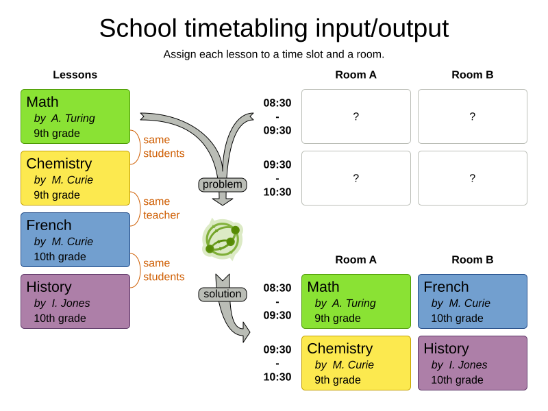
You will build a command-line application that optimizes a school timetable for students and teachers:
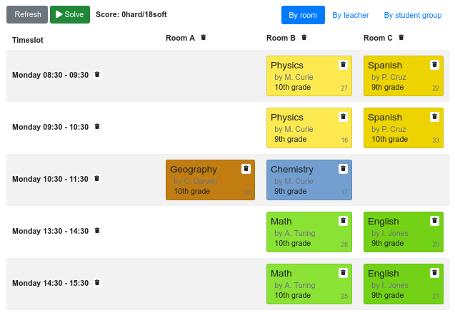
...
INFO  Solving ended: time spent (5000), best score (0hard/9soft), ...
INFO
INFO  |            | Room A     | Room B     | Room C     |
INFO  |------------|------------|------------|------------|
INFO  | MON 08:30  | English    | Math       |            |
INFO  |            | I. Jones   | A. Turing  |            |
INFO  |            | 9th grade  | 10th grade |            |
INFO  |------------|------------|------------|------------|
INFO  | MON 09:30  | History    | Physics    |            |
INFO  |            | I. Jones   | M. Curie   |            |
INFO  |            | 9th grade  | 10th grade |            |
INFO  |------------|------------|------------|------------|
INFO  | MON 10:30  | History    | Physics    |            |
INFO  |            | I. Jones   | M. Curie   |            |
INFO  |            | 10th grade | 9th grade  |            |
INFO  |------------|------------|------------|------------|
...
INFO  |------------|------------|------------|------------|
Your application will assign Lesson instances to Timeslot and Room instances automatically
by using AI to adhere to hard and soft scheduling constraints, for example:
-
A room can have at most one lesson at the same time.
-
A teacher can teach at most one lesson at the same time.
-
A student can attend at most one lesson at the same time.
-
A teacher prefers to teach all lessons in the same room.
-
A teacher prefers to teach sequential lessons and dislikes gaps between lessons.
-
A student dislikes sequential lessons on the same subject.
Mathematically speaking, school timetabling is an NP-hard problem. This means it is difficult to scale. Simply brute force iterating through all possible combinations takes millions of years for a non-trivial dataset, even on a supercomputer. Fortunately, AI constraint solvers such as OptaPlanner have advanced algorithms that deliver a near-optimal solution in a reasonable amount of time.
2.2.2. Solution source code
Follow the instructions in the next sections to create the application step by step (recommended).
Alternatively, review the completed example:
-
Complete one of the following tasks:
-
Clone the Git repository:
$ git clone https://github.com/kiegroup/optaplanner-quickstarts -
Download an archive.
-
-
Find the solution in the
hello-worlddirectory. -
Follow the instructions in the README file to run the application.
2.2.3. Prerequisites
To complete this guide, you need:
-
JDK 11+ with
JAVA_HOMEconfigured appropriately -
Apache Maven 3.8.1+ or Gradle 4+
-
An IDE, such as IntelliJ IDEA, VSCode or Eclipse
2.2.4. The build file and the dependencies
Create a Maven or Gradle build file and add these dependencies:
-
optaplanner-core(compile scope) to solve the school timetable problem. -
optaplanner-test(test scope) to JUnit test the school timetabling constraints. -
A logging implementation, such as
logback-classic(runtime scope), to see what OptaPlanner is doing.
If you choose Maven, your pom.xml file has the following content:
<?xml version="1.0" encoding="UTF-8"?>
<project xmlns="http://maven.apache.org/POM/4.0.0" xmlns:xsi="http://www.w3.org/2001/XMLSchema-instance"
         xsi:schemaLocation="http://maven.apache.org/POM/4.0.0 https://maven.apache.org/xsd/maven-4.0.0.xsd">
  <modelVersion>4.0.0</modelVersion>

  <groupId>org.acme</groupId>
  <artifactId>optaplanner-hello-world-school-timetabling-quickstart</artifactId>
  <version>1.0-SNAPSHOT</version>

  <properties>
    <maven.compiler.release>11</maven.compiler.release>
    <project.build.sourceEncoding>UTF-8</project.build.sourceEncoding>
  </properties>

  <dependencyManagement>
    <dependencies>
      <dependency>
        <groupId>org.optaplanner</groupId>
        <artifactId>optaplanner-bom</artifactId>
        <version>9.44.0.Final</version>
        <type>pom</type>
        <scope>import</scope>
      </dependency>
      <dependency>
        <groupId>ch.qos.logback</groupId>
        <artifactId>logback-classic</artifactId>
        <version>1.2.3</version>
      </dependency>
    </dependencies>
  </dependencyManagement>

  <dependencies>
    <dependency>
      <groupId>org.optaplanner</groupId>
      <artifactId>optaplanner-core</artifactId>
    </dependency>
    <dependency>
      <groupId>ch.qos.logback</groupId>
      <artifactId>logback-classic</artifactId>
      <scope>runtime</scope>
    </dependency>

    <!-- Testing -->
    <dependency>
      <groupId>org.optaplanner</groupId>
      <artifactId>optaplanner-test</artifactId>
      <scope>test</scope>
    </dependency>
  </dependencies>

  <build>
    <plugins>
      <plugin>
        <groupId>org.codehaus.mojo</groupId>
        <artifactId>exec-maven-plugin</artifactId>
        <version>3.0.0</version>
        <configuration>
          <mainClass>org.acme.schooltimetabling.TimeTableApp</mainClass>
        </configuration>
      </plugin>
    </plugins>
  </build>
</project>
On the other hand, in Gradle, your build.gradle file has this content:
plugins {
    id "java"
    id "application"
}

def optaplannerVersion = "9.44.0.Final"
def logbackVersion = "1.2.9"

group = "org.acme"
version = "1.0-SNAPSHOT"

repositories {
    mavenCentral()
}

dependencies {
    implementation platform("org.optaplanner:optaplanner-bom:${optaplannerVersion}")
    implementation "org.optaplanner:optaplanner-core"
    testImplementation "org.optaplanner:optaplanner-test"

    runtimeOnly "ch.qos.logback:logback-classic:${logbackVersion}"
}

java {
    sourceCompatibility = JavaVersion.VERSION_11
    targetCompatibility = JavaVersion.VERSION_11
}

compileJava {
    options.encoding = "UTF-8"
    options.compilerArgs << "-parameters"
}

compileTestJava {
    options.encoding = "UTF-8"
}

application {
    mainClass = "org.acme.schooltimetabling.TimeTableApp"
}

test {
    // Log the test execution results.
    testLogging {
        events "passed", "skipped", "failed"
    }
}
2.2.5. Model the domain objects
Your goal is to assign each lesson to a time slot and a room. You will create these classes:
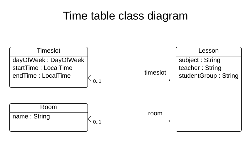
2.2.5.1. Timeslot
The Timeslot class represents a time interval when lessons are taught,
for example, Monday 10:30 - 11:30 or Tuesday 13:30 - 14:30.
For simplicity’s sake, all time slots have the same duration
and there are no time slots during lunch or other breaks.
A time slot has no date, because a high school schedule just repeats every week. So there is no need for continuous planning.
Create the src/main/java/org/acme/schooltimetabling/domain/Timeslot.java class:
package org.acme.schooltimetabling.domain;

import java.time.DayOfWeek;
import java.time.LocalTime;

public class Timeslot {

    private DayOfWeek dayOfWeek;
    private LocalTime startTime;
    private LocalTime endTime;

    public Timeslot() {
    }

    public Timeslot(DayOfWeek dayOfWeek, LocalTime startTime, LocalTime endTime) {
        this.dayOfWeek = dayOfWeek;
        this.startTime = startTime;
        this.endTime = endTime;
    }

    public DayOfWeek getDayOfWeek() {
        return dayOfWeek;
    }

    public LocalTime getStartTime() {
        return startTime;
    }

    public LocalTime getEndTime() {
        return endTime;
    }

    @Override
    public String toString() {
        return dayOfWeek + " " + startTime;
    }

}
Because no Timeslot instances change during solving, a Timeslot is called a problem fact.
Such classes do not require any OptaPlanner specific annotations.
Notice the toString() method keeps the output short,
so it is easier to read OptaPlanner’s DEBUG or TRACE log, as shown later.
2.2.5.2. Room
The Room class represents a location where lessons are taught,
for example, Room A or Room B.
For simplicity’s sake, all rooms are without capacity limits
and they can accommodate all lessons.
Create the src/main/java/org/acme/schooltimetabling/domain/Room.java class:
package org.acme.schooltimetabling.domain;

public class Room {

    private String name;

    public Room() {
    }

    public Room(String name) {
        this.name = name;
    }

    public String getName() {
        return name;
    }

    @Override
    public String toString() {
        return name;
    }

}
Room instances do not change during solving, so Room is also a problem fact.
2.2.5.3. Lesson
During a lesson, represented by the Lesson class,
a teacher teaches a subject to a group of students,
for example, Math by A.Turing for 9th grade or Chemistry by M.Curie for 10th grade.
If a subject is taught multiple times per week by the same teacher to the same student group,
there are multiple Lesson instances that are only distinguishable by id.
For example, the 9th grade has six math lessons a week.
During solving, OptaPlanner changes the timeslot and room fields of the Lesson class,
to assign each lesson to a time slot and a room.
Because OptaPlanner changes these fields, Lesson is a planning entity:
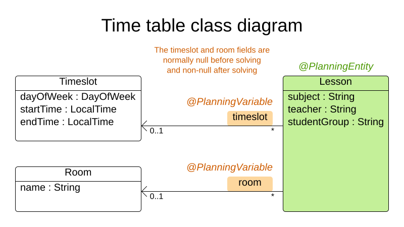
Most of the fields in the previous diagram contain input data, except for the orange fields:
A lesson’s timeslot and room fields are unassigned (null) in the input data
and assigned (not null) in the output data.
OptaPlanner changes these fields during solving.
Such fields are called planning variables.
In order for OptaPlanner to recognize them,
both the timeslot and room fields require an @PlanningVariable annotation.
Their containing class, Lesson, requires an @PlanningEntity annotation.
Create the src/main/java/org/acme/schooltimetabling/domain/Lesson.java class:
package org.acme.schooltimetabling.domain;

import org.optaplanner.core.api.domain.entity.PlanningEntity;
import org.optaplanner.core.api.domain.lookup.PlanningId;
import org.optaplanner.core.api.domain.variable.PlanningVariable;

@PlanningEntity
public class Lesson {

    @PlanningId
    private Long id;

    private String subject;
    private String teacher;
    private String studentGroup;

    @PlanningVariable
    private Timeslot timeslot;
    @PlanningVariable
    private Room room;

    public Lesson() {
    }

    public Lesson(Long id, String subject, String teacher, String studentGroup) {
        this.id = id;
        this.subject = subject;
        this.teacher = teacher;
        this.studentGroup = studentGroup;
    }

    public Long getId() {
        return id;
    }

    public String getSubject() {
        return subject;
    }

    public String getTeacher() {
        return teacher;
    }

    public String getStudentGroup() {
        return studentGroup;
    }

    public Timeslot getTimeslot() {
        return timeslot;
    }

    public void setTimeslot(Timeslot timeslot) {
        this.timeslot = timeslot;
    }

    public Room getRoom() {
        return room;
    }

    public void setRoom(Room room) {
        this.room = room;
    }

    @Override
    public String toString() {
        return subject + "(" + id + ")";
    }

}
The Lesson class has an @PlanningEntity annotation,
so OptaPlanner knows that this class changes during solving
because it contains one or more planning variables.
The timeslot field has an @PlanningVariable annotation,
so OptaPlanner knows that it can change its value.
In order to find potential Timeslot instances to assign to this field,
OptaPlanner uses the variable type to connect to a value range provider
that provides a List<Timeslot> to pick from.
The room field also has an @PlanningVariable annotation, for the same reasons.
|
Determining the |
2.2.6. Define the constraints and calculate the score
A score represents the quality of a specific solution. The higher the better. OptaPlanner looks for the best solution, which is the solution with the highest score found in the available time. It might be the optimal solution.
Because this use case has hard and soft constraints,
use the HardSoftScore class to represent the score:
-
Hard constraints must not be broken. For example: A room can have at most one lesson at the same time.
-
Soft constraints should not be broken. For example: A teacher prefers to teach in a single room.
Hard constraints are weighted against other hard constraints. Soft constraints are weighted too, against other soft constraints. Hard constraints always outweigh soft constraints, regardless of their respective weights.
To calculate the score, you could implement an EasyScoreCalculator class:
public class TimeTableEasyScoreCalculator implements EasyScoreCalculator<TimeTable, HardSoftScore> {

    @Override
    public HardSoftScore calculateScore(TimeTable timeTable) {
        List<Lesson> lessonList = timeTable.getLessonList();
        int hardScore = 0;
        for (Lesson a : lessonList) {
            for (Lesson b : lessonList) {
                if (a.getTimeslot() != null && a.getTimeslot().equals(b.getTimeslot())
                        && a.getId() < b.getId()) {
                    // A room can accommodate at most one lesson at the same time.
                    if (a.getRoom() != null && a.getRoom().equals(b.getRoom())) {
                        hardScore--;
                    }
                    // A teacher can teach at most one lesson at the same time.
                    if (a.getTeacher().equals(b.getTeacher())) {
                        hardScore--;
                    }
                    // A student can attend at most one lesson at the same time.
                    if (a.getStudentGroup().equals(b.getStudentGroup())) {
                        hardScore--;
                    }
                }
            }
        }
        int softScore = 0;
        // Soft constraints are only implemented in the optaplanner-quickstarts code
        return HardSoftScore.of(hardScore, softScore);
    }

}
Unfortunately that does not scale well, because it is non-incremental: every time a lesson is assigned to a different time slot or room, all lessons are re-evaluated to calculate the new score.
Instead, create a src/main/java/org/acme/schooltimetabling/solver/TimeTableConstraintProvider.java class
to perform incremental score calculation.
It uses OptaPlanner’s ConstraintStream API which is inspired by Java Streams and SQL:
package org.acme.schooltimetabling.solver;

import org.acme.schooltimetabling.domain.Lesson;
import org.optaplanner.core.api.score.buildin.hardsoft.HardSoftScore;
import org.optaplanner.core.api.score.stream.Constraint;
import org.optaplanner.core.api.score.stream.ConstraintFactory;
import org.optaplanner.core.api.score.stream.ConstraintProvider;
import org.optaplanner.core.api.score.stream.Joiners;

public class TimeTableConstraintProvider implements ConstraintProvider {

    @Override
    public Constraint[] defineConstraints(ConstraintFactory constraintFactory) {
        return new Constraint[] {
                // Hard constraints
                roomConflict(constraintFactory),
                teacherConflict(constraintFactory),
                studentGroupConflict(constraintFactory),
                // Soft constraints are only implemented in the optaplanner-quickstarts code
        };
    }

    private Constraint roomConflict(ConstraintFactory constraintFactory) {
        // A room can accommodate at most one lesson at the same time.

        // Select a lesson ...
        return constraintFactory
                .forEach(Lesson.class)
                // ... and pair it with another lesson ...
                .join(Lesson.class,
                        // ... in the same timeslot ...
                        Joiners.equal(Lesson::getTimeslot),
                        // ... in the same room ...
                        Joiners.equal(Lesson::getRoom),
                        // ... and the pair is unique (different id, no reverse pairs) ...
                        Joiners.lessThan(Lesson::getId))
                // ... then penalize each pair with a hard weight.
                .penalize(HardSoftScore.ONE_HARD)
                .asConstraint("Room conflict");
    }

    private Constraint teacherConflict(ConstraintFactory constraintFactory) {
        // A teacher can teach at most one lesson at the same time.
        return constraintFactory.forEach(Lesson.class)
                .join(Lesson.class,
                        Joiners.equal(Lesson::getTimeslot),
                        Joiners.equal(Lesson::getTeacher),
                        Joiners.lessThan(Lesson::getId))
                .penalize(HardSoftScore.ONE_HARD)
                .asConstraint("Teacher conflict");
    }

    private Constraint studentGroupConflict(ConstraintFactory constraintFactory) {
        // A student can attend at most one lesson at the same time.
        return constraintFactory.forEach(Lesson.class)
                .join(Lesson.class,
                        Joiners.equal(Lesson::getTimeslot),
                        Joiners.equal(Lesson::getStudentGroup),
                        Joiners.lessThan(Lesson::getId))
                .penalize(HardSoftScore.ONE_HARD)
                .asConstraint("Student group conflict");
    }

}
The ConstraintProvider scales an order of magnitude better than the EasyScoreCalculator: O(n) instead of O(n²).
2.2.7. Gather the domain objects in a planning solution
A TimeTable wraps all Timeslot, Room, and Lesson instances of a single dataset.
Furthermore, because it contains all lessons, each with a specific planning variable state,
it is a planning solution and it has a score:
-
If lessons are still unassigned, then it is an uninitialized solution, for example, a solution with the score
-4init/0hard/0soft. -
If it breaks hard constraints, then it is an infeasible solution, for example, a solution with the score
-2hard/-3soft. -
If it adheres to all hard constraints, then it is a feasible solution, for example, a solution with the score
0hard/-7soft.
Create the src/main/java/org/acme/schooltimetabling/domain/TimeTable.java class:
package org.acme.schooltimetabling.domain;

import java.util.List;

import org.optaplanner.core.api.domain.solution.PlanningEntityCollectionProperty;
import org.optaplanner.core.api.domain.solution.PlanningScore;
import org.optaplanner.core.api.domain.solution.PlanningSolution;
import org.optaplanner.core.api.domain.solution.ProblemFactCollectionProperty;
import org.optaplanner.core.api.domain.valuerange.ValueRangeProvider;
import org.optaplanner.core.api.score.buildin.hardsoft.HardSoftScore;

@PlanningSolution
public class TimeTable {

    @ValueRangeProvider
    @ProblemFactCollectionProperty
    private List<Timeslot> timeslotList;
    @ValueRangeProvider
    @ProblemFactCollectionProperty
    private List<Room> roomList;
    @PlanningEntityCollectionProperty
    private List<Lesson> lessonList;

    @PlanningScore
    private HardSoftScore score;

    public TimeTable() {
    }

    public TimeTable(List<Timeslot> timeslotList, List<Room> roomList, List<Lesson> lessonList) {
        this.timeslotList = timeslotList;
        this.roomList = roomList;
        this.lessonList = lessonList;
    }

    public List<Timeslot> getTimeslotList() {
        return timeslotList;
    }

    public List<Room> getRoomList() {
        return roomList;
    }

    public List<Lesson> getLessonList() {
        return lessonList;
    }

    public HardSoftScore getScore() {
        return score;
    }

}
The TimeTable class has an @PlanningSolution annotation,
so OptaPlanner knows that this class contains all of the input and output data.
Specifically, this class is the input of the problem:
-
A
timeslotListfield with all time slots-
This is a list of problem facts, because they do not change during solving.
-
-
A
roomListfield with all rooms-
This is a list of problem facts, because they do not change during solving.
-
-
A
lessonListfield with all lessons-
This is a list of planning entities, because they change during solving.
-
Of each
Lesson:-
The values of the
timeslotandroomfields are typically stillnull, so unassigned. They are planning variables. -
The other fields, such as
subject,teacherandstudentGroup, are filled in. These fields are problem properties.
-
-
However, this class is also the output of the solution:
-
A
lessonListfield for which eachLessoninstance has non-nulltimeslotandroomfields after solving -
A
scorefield that represents the quality of the output solution, for example,0hard/-5soft
2.2.7.1. The value range providers
The timeslotList field is a value range provider.
It holds the Timeslot instances which OptaPlanner can pick from to assign to the timeslot field of Lesson instances.
The timeslotList field has an @ValueRangeProvider annotation to connect the @PlanningVariable with the @ValueRangeProvider,
by matching the type of the planning variable with the type returned by the value range provider.
Following the same logic, the roomList field also has an @ValueRangeProvider annotation.
2.2.7.2. The problem fact and planning entity properties
Furthermore, OptaPlanner needs to know which Lesson instances it can change
as well as how to retrieve the Timeslot and Room instances used for score calculation
by your TimeTableConstraintProvider.
The timeslotList and roomList fields have an @ProblemFactCollectionProperty annotation,
so your TimeTableConstraintProvider can select from those instances.
The lessonList has an @PlanningEntityCollectionProperty annotation,
so OptaPlanner can change them during solving
and your TimeTableConstraintProvider can select from those too.
2.2.8. Create the application
Now you are ready to put everything together and create a Java application.
The main() method performs the following tasks:
-
Creates the
SolverFactoryto build aSolverper dataset. -
Loads a dataset.
-
Solves it with
Solver.solve(). -
Visualizes the solution for that dataset.
Typically, an application has a single SolverFactory
to build a new Solver instance for each problem dataset to solve.
A SolverFactory is thread-safe, but a Solver is not.
In this case, there is only one dataset, so only one Solver instance.
Create the src/main/java/org/acme/schooltimetabling/TimeTableApp.java class:
package org.acme.schooltimetabling;

import java.time.DayOfWeek;
import java.time.Duration;
import java.time.LocalTime;
import java.util.ArrayList;
import java.util.Collections;
import java.util.List;
import java.util.Map;
import java.util.stream.Collectors;

import org.acme.schooltimetabling.domain.Lesson;
import org.acme.schooltimetabling.domain.Room;
import org.acme.schooltimetabling.domain.TimeTable;
import org.acme.schooltimetabling.domain.Timeslot;
import org.acme.schooltimetabling.solver.TimeTableConstraintProvider;
import org.optaplanner.core.api.solver.Solver;
import org.optaplanner.core.api.solver.SolverFactory;
import org.optaplanner.core.config.solver.SolverConfig;
import org.slf4j.Logger;
import org.slf4j.LoggerFactory;

public class TimeTableApp {

    private static final Logger LOGGER = LoggerFactory.getLogger(TimeTableApp.class);

    public static void main(String[] args) {
        SolverFactory<TimeTable> solverFactory = SolverFactory.create(new SolverConfig()
                .withSolutionClass(TimeTable.class)
                .withEntityClasses(Lesson.class)
                .withConstraintProviderClass(TimeTableConstraintProvider.class)
                // The solver runs only for 5 seconds on this small dataset.
                // It's recommended to run for at least 5 minutes ("5m") otherwise.
                .withTerminationSpentLimit(Duration.ofSeconds(5)));

        // Load the problem
        TimeTable problem = generateDemoData();

        // Solve the problem
        Solver<TimeTable> solver = solverFactory.buildSolver();
        TimeTable solution = solver.solve(problem);

        // Visualize the solution
        printTimetable(solution);
    }

    public static TimeTable generateDemoData() {
        List<Timeslot> timeslotList = new ArrayList<>(10);
        timeslotList.add(new Timeslot(DayOfWeek.MONDAY, LocalTime.of(8, 30), LocalTime.of(9, 30)));
        timeslotList.add(new Timeslot(DayOfWeek.MONDAY, LocalTime.of(9, 30), LocalTime.of(10, 30)));
        timeslotList.add(new Timeslot(DayOfWeek.MONDAY, LocalTime.of(10, 30), LocalTime.of(11, 30)));
        timeslotList.add(new Timeslot(DayOfWeek.MONDAY, LocalTime.of(13, 30), LocalTime.of(14, 30)));
        timeslotList.add(new Timeslot(DayOfWeek.MONDAY, LocalTime.of(14, 30), LocalTime.of(15, 30)));

        timeslotList.add(new Timeslot(DayOfWeek.TUESDAY, LocalTime.of(8, 30), LocalTime.of(9, 30)));
        timeslotList.add(new Timeslot(DayOfWeek.TUESDAY, LocalTime.of(9, 30), LocalTime.of(10, 30)));
        timeslotList.add(new Timeslot(DayOfWeek.TUESDAY, LocalTime.of(10, 30), LocalTime.of(11, 30)));
        timeslotList.add(new Timeslot(DayOfWeek.TUESDAY, LocalTime.of(13, 30), LocalTime.of(14, 30)));
        timeslotList.add(new Timeslot(DayOfWeek.TUESDAY, LocalTime.of(14, 30), LocalTime.of(15, 30)));

        List<Room> roomList = new ArrayList<>(3);
        roomList.add(new Room("Room A"));
        roomList.add(new Room("Room B"));
        roomList.add(new Room("Room C"));

        List<Lesson> lessonList = new ArrayList<>();
        long id = 0;
        lessonList.add(new Lesson(id++, "Math", "A. Turing", "9th grade"));
        lessonList.add(new Lesson(id++, "Math", "A. Turing", "9th grade"));
        lessonList.add(new Lesson(id++, "Physics", "M. Curie", "9th grade"));
        lessonList.add(new Lesson(id++, "Chemistry", "M. Curie", "9th grade"));
        lessonList.add(new Lesson(id++, "Biology", "C. Darwin", "9th grade"));
        lessonList.add(new Lesson(id++, "History", "I. Jones", "9th grade"));
        lessonList.add(new Lesson(id++, "English", "I. Jones", "9th grade"));
        lessonList.add(new Lesson(id++, "English", "I. Jones", "9th grade"));
        lessonList.add(new Lesson(id++, "Spanish", "P. Cruz", "9th grade"));
        lessonList.add(new Lesson(id++, "Spanish", "P. Cruz", "9th grade"));

        lessonList.add(new Lesson(id++, "Math", "A. Turing", "10th grade"));
        lessonList.add(new Lesson(id++, "Math", "A. Turing", "10th grade"));
        lessonList.add(new Lesson(id++, "Math", "A. Turing", "10th grade"));
        lessonList.add(new Lesson(id++, "Physics", "M. Curie", "10th grade"));
        lessonList.add(new Lesson(id++, "Chemistry", "M. Curie", "10th grade"));
        lessonList.add(new Lesson(id++, "French", "M. Curie", "10th grade"));
        lessonList.add(new Lesson(id++, "Geography", "C. Darwin", "10th grade"));
        lessonList.add(new Lesson(id++, "History", "I. Jones", "10th grade"));
        lessonList.add(new Lesson(id++, "English", "P. Cruz", "10th grade"));
        lessonList.add(new Lesson(id++, "Spanish", "P. Cruz", "10th grade"));

        return new TimeTable(timeslotList, roomList, lessonList);
    }

    private static void printTimetable(TimeTable timeTable) {
        LOGGER.info("");
        List<Room> roomList = timeTable.getRoomList();
        List<Lesson> lessonList = timeTable.getLessonList();
        Map<Timeslot, Map<Room, List<Lesson>>> lessonMap = lessonList.stream()
                .filter(lesson -> lesson.getTimeslot() != null && lesson.getRoom() != null)
                .collect(Collectors.groupingBy(Lesson::getTimeslot, Collectors.groupingBy(Lesson::getRoom)));
        LOGGER.info("|            | " + roomList.stream()
                .map(room -> String.format("%-10s", room.getName())).collect(Collectors.joining(" | ")) + " |");
        LOGGER.info("|" + "------------|".repeat(roomList.size() + 1));
        for (Timeslot timeslot : timeTable.getTimeslotList()) {
            List<List<Lesson>> cellList = roomList.stream()
                    .map(room -> {
                        Map<Room, List<Lesson>> byRoomMap = lessonMap.get(timeslot);
                        if (byRoomMap == null) {
                            return Collections.<Lesson>emptyList();
                        }
                        List<Lesson> cellLessonList = byRoomMap.get(room);
                        if (cellLessonList == null) {
                            return Collections.<Lesson>emptyList();
                        }
                        return cellLessonList;
                    })
                    .collect(Collectors.toList());

            LOGGER.info("| " + String.format("%-10s",
                    timeslot.getDayOfWeek().toString().substring(0, 3) + " " + timeslot.getStartTime()) + " | "
                    + cellList.stream().map(cellLessonList -> String.format("%-10s",
                            cellLessonList.stream().map(Lesson::getSubject).collect(Collectors.joining(", "))))
                            .collect(Collectors.joining(" | "))
                    + " |");
            LOGGER.info("|            | "
                    + cellList.stream().map(cellLessonList -> String.format("%-10s",
                            cellLessonList.stream().map(Lesson::getTeacher).collect(Collectors.joining(", "))))
                            .collect(Collectors.joining(" | "))
                    + " |");
            LOGGER.info("|            | "
                    + cellList.stream().map(cellLessonList -> String.format("%-10s",
                            cellLessonList.stream().map(Lesson::getStudentGroup).collect(Collectors.joining(", "))))
                            .collect(Collectors.joining(" | "))
                    + " |");
            LOGGER.info("|" + "------------|".repeat(roomList.size() + 1));
        }
        List<Lesson> unassignedLessons = lessonList.stream()
                .filter(lesson -> lesson.getTimeslot() == null || lesson.getRoom() == null)
                .collect(Collectors.toList());
        if (!unassignedLessons.isEmpty()) {
            LOGGER.info("");
            LOGGER.info("Unassigned lessons");
            for (Lesson lesson : unassignedLessons) {
                LOGGER.info("  " + lesson.getSubject() + " - " + lesson.getTeacher() + " - " + lesson.getStudentGroup());
            }
        }
    }

}
The main() method first creates the SolverFactory:
SolverFactory<TimeTable> solverFactory = SolverFactory.create(new SolverConfig()
        .withSolutionClass(TimeTable.class)
        .withEntityClasses(Lesson.class)
        .withConstraintProviderClass(TimeTableConstraintProvider.class)
        // The solver runs only for 5 seconds on this small dataset.
        // It's recommended to run for at least 5 minutes ("5m") otherwise.
        .withTerminationSpentLimit(Duration.ofSeconds(5)));
This registers the @PlanningSolution class, the @PlanningEntity classes,
and the ConstraintProvider class, all of which you created earlier.
Without a termination setting or a terminationEarly() event, the solver runs forever.
To avoid that, the solver limits the solving time to five seconds.
After five seconds, the main() method loads the problem, solves it, and prints the solution:
        // Load the problem
        TimeTable problem = generateDemoData();

        // Solve the problem
        Solver<TimeTable> solver = solverFactory.buildSolver();
        TimeTable solution = solver.solve(problem);

        // Visualize the solution
        printTimetable(solution);
The solve() method doesn’t return instantly.
It runs for five seconds before returning the best solution.
OptaPlanner returns the best solution found in the available termination time. Due to the nature of NP-hard problems, the best solution might not be optimal, especially for larger datasets. Increase the termination time to potentially find a better solution.
The generateDemoData() method generates the school timetable problem to solve.
The printTimetable() method pretty prints the timetable to the console,
so it’s easy to determine visually whether or not it’s a good schedule.
2.2.8.1. Configure logging
To see any output in the console, logging must be configured properly.
Create the src/main/resource/logback.xml file:
<?xml version="1.0" encoding="UTF-8"?>
<configuration>

  <appender name="consoleAppender" class="ch.qos.logback.core.ConsoleAppender">
    <encoder>
      <pattern>%d{HH:mm:ss.SSS} [%-12.12t] %-5p %m%n</pattern>
    </encoder>
  </appender>

  <logger name="org.optaplanner" level="info"/>

  <root level="info">
    <appender-ref ref="consoleAppender" />
  </root>

</configuration>
2.2.9. Run the application
2.2.9.1. Run the application in IDE
Run that TimeTableApp class as the main class of a normal Java application:
...
INFO  |            | Room A     | Room B     | Room C     |
INFO  |------------|------------|------------|------------|
INFO  | MON 08:30  | English    | Math       |            |
INFO  |            | I. Jones   | A. Turing  |            |
INFO  |            | 9th grade  | 10th grade |            |
INFO  |------------|------------|------------|------------|
INFO  | MON 09:30  | History    | Physics    |            |
INFO  |            | I. Jones   | M. Curie   |            |
INFO  |            | 9th grade  | 10th grade |            |
...
Verify the console output. Does it conform to all hard constraints?
What happens if you comment out the roomConflict constraint in TimeTableConstraintProvider?
The info log shows what OptaPlanner did in those five seconds:
... Solving started: time spent (33), best score (-8init/0hard/0soft), environment mode (REPRODUCIBLE), random (JDK with seed 0).
... Construction Heuristic phase (0) ended: time spent (73), best score (0hard/0soft), score calculation speed (459/sec), step total (4).
... Local Search phase (1) ended: time spent (5000), best score (0hard/0soft), score calculation speed (28949/sec), step total (28398).
... Solving ended: time spent (5000), best score (0hard/0soft), score calculation speed (28524/sec), phase total (2), environment mode (REPRODUCIBLE).
2.2.9.2. Test the application
A good application includes test coverage.
2.2.9.2.1. Test the constraints
To test each constraint in isolation, use a ConstraintVerifier in unit tests.
This tests each constraint’s corner cases in isolation from the other tests,
which lowers maintenance when adding a new constraint with proper test coverage.
Create the src/test/java/org/acme/schooltimetabling/solver/TimeTableConstraintProviderTest.java class:
package org.acme.schooltimetabling.solver;

import java.time.DayOfWeek;
import java.time.LocalTime;

import org.acme.schooltimetabling.domain.Lesson;
import org.acme.schooltimetabling.domain.Room;
import org.acme.schooltimetabling.domain.TimeTable;
import org.acme.schooltimetabling.domain.Timeslot;
import org.junit.jupiter.api.Test;
import org.optaplanner.test.api.score.stream.ConstraintVerifier;

class TimeTableConstraintProviderTest {

    private static final Room ROOM1 = new Room("Room1");
    private static final Timeslot TIMESLOT1 = new Timeslot(DayOfWeek.MONDAY, LocalTime.NOON);
    private static final Timeslot TIMESLOT2 = new Timeslot(DayOfWeek.TUESDAY, LocalTime.NOON);

    ConstraintVerifier<TimeTableConstraintProvider, TimeTable> constraintVerifier = ConstraintVerifier.build(
            new TimeTableConstraintProvider(), TimeTable.class, Lesson.class);

    @Test
    void roomConflict() {
        Lesson firstLesson = new Lesson(1, "Subject1", "Teacher1", "Group1", TIMESLOT1, ROOM1);
        Lesson conflictingLesson = new Lesson(2, "Subject2", "Teacher2", "Group2", TIMESLOT1, ROOM1);
        Lesson nonConflictingLesson = new Lesson(3, "Subject3", "Teacher3", "Group3", TIMESLOT2, ROOM1);
        constraintVerifier.verifyThat(TimeTableConstraintProvider::roomConflict)
                .given(firstLesson, conflictingLesson, nonConflictingLesson)
                .penalizesBy(1);
    }

}
This test verifies that the constraint TimeTableConstraintProvider::roomConflict penalizes with a match weight of 1
when given three lessons in the same room, where two lessons have the same timeslot.
Therefore, a constraint weight of 10hard would reduce the score by -10hard.
Notice how ConstraintVerifier ignores the constraint weight during testing - even
if those constraint weights are hard coded in the ConstraintProvider - because
constraints weights change regularly before going into production.
This way, constraint weight tweaking does not break the unit tests.
For more, see Testing Constraint Streams.
2.2.9.3. Logging
When adding constraints in your ConstraintProvider,
keep an eye on the score calculation speed in the info log,
after solving for the same amount of time, to assess the performance impact:
... Solving ended: ..., score calculation speed (29455/sec), ...To understand how OptaPlanner is solving your problem internally,
change the logging in the logback.xml file:
<logger name="org.optaplanner" level="debug"/>Use debug logging to show every step:
... Solving started: time spent (67), best score (-20init/0hard/0soft), environment mode (REPRODUCIBLE), random (JDK with seed 0).
...     CH step (0), time spent (128), score (-18init/0hard/0soft), selected move count (15), picked move ([Math(101) {null -> Room A}, Math(101) {null -> MONDAY 08:30}]).
...     CH step (1), time spent (145), score (-16init/0hard/0soft), selected move count (15), picked move ([Physics(102) {null -> Room A}, Physics(102) {null -> MONDAY 09:30}]).
...
Use trace logging to show every step and every move per step.
2.2.9.4. Make a standalone application
In order to run the application outside an IDE easily, you will need to make some changes to the configuration of your build tool.
2.2.9.4.1. Executable JAR in Maven
In Maven, add the following to your pom.xml:
  ...
  <build>
    <plugins>
      <plugin>
        <groupId>org.apache.maven.plugins</groupId>
        <artifactId>maven-assembly-plugin</artifactId>
        <version>${version.assembly.plugin}</version>
        <configuration>
          <finalName>hello-world-run</finalName>
          <appendAssemblyId>false</appendAssemblyId>
          <descriptors>
            <descriptor>src/assembly/jar-with-dependencies-and-services.xml</descriptor>
          </descriptors>
          <archive>
            <manifestEntries>
              <Main-Class>org.acme.schooltimetabling.TimeTableApp</Main-Class>
              <Multi-Release>true</Multi-Release>
            </manifestEntries>
          </archive>
        </configuration>
        <executions>
          <execution>
            <id>make-assembly</id>
            <phase>package</phase>
            <goals>
              <goal>single</goal>
            </goals>
          </execution>
        </executions>
      </plugin>
      ...
    </plugins>
    ...
  </build>
  ...
Also, create a new file in src/assembly directory called jar-with-dependencies-and-services.xml with the following contents:
  <assembly xmlns="http://maven.apache.org/ASSEMBLY/2.1.0"
            xmlns:xsi="http://www.w3.org/2001/XMLSchema-instance"
            xsi:schemaLocation="http://maven.apache.org/ASSEMBLY/2.1.0 http://maven.apache.org/xsd/assembly-2.1.0.xsd">
    <id>jar-with-dependencies-and-services</id>
    <formats>
      <format>jar</format>
    </formats>
    <containerDescriptorHandlers>
      <containerDescriptorHandler>
        <handlerName>metaInf-services</handlerName>
      </containerDescriptorHandler>
    </containerDescriptorHandlers>
    <includeBaseDirectory>false</includeBaseDirectory>
    <dependencySets>
      <dependencySet>
        <outputDirectory>/</outputDirectory>
        <useProjectArtifact>true</useProjectArtifact>
        <unpack>true</unpack>
        <scope>runtime</scope>
      </dependencySet>
    </dependencySets>
  </assembly>
This enables the Maven Assembly Plugin and tells it to do the following:
-
Take all dependencies of your project and put their classes and resources into a new JAR.
-
If any of the dependencies use Java SPI, it properly bundles all the service descriptors.
-
If any of the dependencies are multi-release JARs, it takes that into account.
-
-
Set that JAR’s main class to be
org.acme.schooltimetabling.TimeTableApp. -
Make that JAR available as
hello-world-run.jarin your project’s build directory, most likelytarget/.
This executable JAR can be run like any other JAR:
$ mvn clean install
...
$ java -jar target/hello-world-run.jar
2.2.9.4.2. Executable application in Gradle
In Gradle, add the following to your build.gradle:
application {
    mainClass = "org.acme.schooltimetabling.TimeTableApp"
}
After building the project, you can find an archive with a runnable application inside the build/distributions/ directory.
2.2.10. Summary
Congratulations! You have just developed a Java application with OptaPlanner!
If you ran into any issues, take a look at the quickstart source code.
Read the next guide to build a pretty web application for school timetabling with a REST service and database integration, by leveraging Quarkus.
2.3. Quarkus Java quick start
This guide walks you through the process of creating a Quarkus application with OptaPlanner's constraint solving Artificial Intelligence (AI).
2.3.1. What you will build
You will build a REST application that optimizes a school timetable for students and teachers:
Your service will assign Lesson instances to Timeslot and Room instances automatically
by using AI to adhere to hard and soft scheduling constraints, such as the following examples:
-
A room can have at most one lesson at the same time.
-
A teacher can teach at most one lesson at the same time.
-
A student can attend at most one lesson at the same time.
-
A teacher prefers to teach all lessons in the same room.
-
A teacher prefers to teach sequential lessons and dislikes gaps between lessons.
-
A student dislikes sequential lessons on the same subject.
Mathematically speaking, school timetabling is an NP-hard problem. This means it is difficult to scale. Simply brute force iterating through all possible combinations takes millions of years for a non-trivial dataset, even on a supercomputer. Luckily, AI constraint solvers such as OptaPlanner have advanced algorithms that deliver a near-optimal solution in a reasonable amount of time.
2.3.2. Solution source code
Follow the instructions in the next sections to create the application step by step (recommended).
Alternatively, you can also skip right to the completed example:
-
Clone the Git repository:
$ git clone https://github.com/kiegroup/optaplanner-quickstartsor download an archive.
-
Find the solution in the
use-casesdirectory and run it (see its README file).
2.3.3. Prerequisites
To complete this guide, you need:
-
JDK 11+ with
JAVA_HOMEconfigured appropriately -
Apache Maven 3.8.1+ or Gradle 4+
-
An IDE, such as IntelliJ IDEA, VSCode or Eclipse
2.3.4. The build file and the dependencies
Use code.quarkus.io to generate an application with the following extensions, for Maven or Gradle:
-
RESTEasy JAX-RS (
quarkus-resteasy) -
RESTEasy Jackson (
quarkus-resteasy-jackson) -
OptaPlanner (
optaplanner-quarkus) -
OptaPlanner Jackson (
optaplanner-quarkus-jackson)
Alternatively, generate it from the command line with Maven:
$ mvn io.quarkus:quarkus-maven-plugin:3.0.0.Final:create \
    -DprojectGroupId=org.acme \
    -DprojectArtifactId=optaplanner-quickstart \
    -Dextensions="resteasy,resteasy-jackson,optaplanner-quarkus,optaplanner-quarkus-jackson" \
    -DnoExamples
$ cd optaplanner-quickstart
If you choose Maven, your pom.xml file has the following content:
<?xml version="1.0" encoding="UTF-8"?>
<project xmlns="http://maven.apache.org/POM/4.0.0" xmlns:xsi="http://www.w3.org/2001/XMLSchema-instance"
         xsi:schemaLocation="http://maven.apache.org/POM/4.0.0 https://maven.apache.org/xsd/maven-4.0.0.xsd">
  <modelVersion>4.0.0</modelVersion>

  <groupId>org.acme</groupId>
  <artifactId>optaplanner-quarkus-school-timetabling-quickstart</artifactId>
  <version>1.0-SNAPSHOT</version>

  <properties>
    <maven.compiler.release>11</maven.compiler.release>
    <project.build.sourceEncoding>UTF-8</project.build.sourceEncoding>

    <version.io.quarkus>3.0.0.Final</version.io.quarkus>
    <version.org.optaplanner>9.44.0.Final</version.org.optaplanner>
  </properties>

  <dependencyManagement>
    <dependencies>
      <dependency>
        <groupId>io.quarkus</groupId>
        <artifactId>quarkus-bom</artifactId>
        <version>${version.io.quarkus}</version>
        <type>pom</type>
        <scope>import</scope>
      </dependency>
      <dependency>
        <groupId>org.optaplanner</groupId>
        <artifactId>optaplanner-bom</artifactId>
        <version>${version.org.optaplanner}</version>
        <type>pom</type>
        <scope>import</scope>
      </dependency>
    </dependencies>
  </dependencyManagement>
  <dependencies>
    <dependency>
      <groupId>io.quarkus</groupId>
      <artifactId>quarkus-resteasy</artifactId>
    </dependency>
    <dependency>
      <groupId>io.quarkus</groupId>
      <artifactId>quarkus-resteasy-jackson</artifactId>
    </dependency>
    <dependency>
      <groupId>org.optaplanner</groupId>
      <artifactId>optaplanner-quarkus</artifactId>
    </dependency>
    <dependency>
      <groupId>org.optaplanner</groupId>
      <artifactId>optaplanner-quarkus-jackson</artifactId>
    </dependency>

    <dependency>
      <groupId>io.quarkus</groupId>
      <artifactId>quarkus-junit5</artifactId>
      <scope>test</scope>
    </dependency>
    <dependency>
      <groupId>org.optaplanner</groupId>
      <artifactId>optaplanner-test</artifactId>
      <scope>test</scope>
    </dependency>
  </dependencies>

  <build>
    <plugins>
      <plugin>
        <groupId>io.quarkus</groupId>
        <artifactId>quarkus-maven-plugin</artifactId>
        <version>${version.io.quarkus}</version>
        <executions>
          <execution>
            <goals>
              <goal>build</goal>
            </goals>
          </execution>
        </executions>
      </plugin>
      <plugin>
        <artifactId>maven-surefire-plugin</artifactId>
        <configuration>
          <systemPropertyVariables>
            <java.util.logging.manager>org.jboss.logmanager.LogManager</java.util.logging.manager>
          </systemPropertyVariables>
        </configuration>
      </plugin>
    </plugins>
  </build>
</project>
On the other hand, in Gradle, your build.gradle file has this content:
plugins {
    id "java"
    id "io.quarkus" version "3.0.0.Final"
}

def quarkusVersion = "3.0.0.Final"
def optaplannerVersion = "9.44.0.Final"

group = "org.acme"
version = "1.0-SNAPSHOT"

repositories {
    mavenCentral()
}

dependencies {
    implementation platform("io.quarkus:quarkus-bom:${quarkusVersion}")
    implementation "io.quarkus:quarkus-resteasy"
    implementation "io.quarkus:quarkus-resteasy-jackson"
    testImplementation "io.quarkus:quarkus-junit5"

    implementation platform("org.optaplanner:optaplanner-bom:${optaplannerVersion}")
    implementation "org.optaplanner:optaplanner-quarkus"
    implementation "org.optaplanner:optaplanner-quarkus-jackson"
    testImplementation "org.optaplanner:optaplanner-test"
}

java {
    sourceCompatibility = JavaVersion.VERSION_11
    targetCompatibility = JavaVersion.VERSION_11
}

compileJava {
    options.encoding = "UTF-8"
    options.compilerArgs << "-parameters"
}

compileTestJava {
    options.encoding = "UTF-8"
}

test {
    systemProperty "java.util.logging.manager", "org.jboss.logmanager.LogManager"
}
2.3.5. Model the domain objects
Your goal is to assign each lesson to a time slot and a room. You will create these classes:
2.3.5.1. Timeslot
The Timeslot class represents a time interval when lessons are taught,
for example, Monday 10:30 - 11:30 or Tuesday 13:30 - 14:30.
For simplicity’s sake, all time slots have the same duration
and there are no time slots during lunch or other breaks.
A time slot has no date, because a high school schedule just repeats every week. So there is no need for continuous planning.
Create the src/main/java/org/acme/schooltimetabling/domain/Timeslot.java class:
package org.acme.schooltimetabling.domain;

import java.time.DayOfWeek;
import java.time.LocalTime;

public class Timeslot {

    private DayOfWeek dayOfWeek;
    private LocalTime startTime;
    private LocalTime endTime;

    public Timeslot() {
    }

    public Timeslot(DayOfWeek dayOfWeek, LocalTime startTime, LocalTime endTime) {
        this.dayOfWeek = dayOfWeek;
        this.startTime = startTime;
        this.endTime = endTime;
    }

    public DayOfWeek getDayOfWeek() {
        return dayOfWeek;
    }

    public LocalTime getStartTime() {
        return startTime;
    }

    public LocalTime getEndTime() {
        return endTime;
    }

    @Override
    public String toString() {
        return dayOfWeek + " " + startTime;
    }

}
Because no Timeslot instances change during solving, a Timeslot is called a problem fact.
Such classes do not require any OptaPlanner specific annotations.
Notice the toString() method keeps the output short,
so it is easier to read OptaPlanner’s DEBUG or TRACE log, as shown later.
2.3.5.2. Room
The Room class represents a location where lessons are taught,
for example, Room A or Room B.
For simplicity’s sake, all rooms are without capacity limits
and they can accommodate all lessons.
Create the src/main/java/org/acme/schooltimetabling/domain/Room.java class:
package org.acme.schooltimetabling.domain;

public class Room {

    private String name;

    public Room() {
    }

    public Room(String name) {
        this.name = name;
    }

    public String getName() {
        return name;
    }

    @Override
    public String toString() {
        return name;
    }

}
Room instances do not change during solving, so Room is also a problem fact.
2.3.5.3. Lesson
During a lesson, represented by the Lesson class,
a teacher teaches a subject to a group of students,
for example, Math by A.Turing for 9th grade or Chemistry by M.Curie for 10th grade.
If a subject is taught multiple times per week by the same teacher to the same student group,
there are multiple Lesson instances that are only distinguishable by id.
For example, the 9th grade has six math lessons a week.
During solving, OptaPlanner changes the timeslot and room fields of the Lesson class,
to assign each lesson to a time slot and a room.
Because OptaPlanner changes these fields, Lesson is a planning entity:
Most of the fields in the previous diagram contain input data, except for the orange fields:
A lesson’s timeslot and room fields are unassigned (null) in the input data
and assigned (not null) in the output data.
OptaPlanner changes these fields during solving.
Such fields are called planning variables.
In order for OptaPlanner to recognize them,
both the timeslot and room fields require an @PlanningVariable annotation.
Their containing class, Lesson, requires an @PlanningEntity annotation.
Create the src/main/java/org/acme/schooltimetabling/domain/Lesson.java class:
package org.acme.schooltimetabling.domain;

import org.optaplanner.core.api.domain.entity.PlanningEntity;
import org.optaplanner.core.api.domain.lookup.PlanningId;
import org.optaplanner.core.api.domain.variable.PlanningVariable;

@PlanningEntity
public class Lesson {

    @PlanningId
    private Long id;

    private String subject;
    private String teacher;
    private String studentGroup;

    @PlanningVariable
    private Timeslot timeslot;
    @PlanningVariable
    private Room room;

    public Lesson() {
    }

    public Lesson(Long id, String subject, String teacher, String studentGroup) {
        this.id = id;
        this.subject = subject;
        this.teacher = teacher;
        this.studentGroup = studentGroup;
    }

    public Long getId() {
        return id;
    }

    public String getSubject() {
        return subject;
    }

    public String getTeacher() {
        return teacher;
    }

    public String getStudentGroup() {
        return studentGroup;
    }

    public Timeslot getTimeslot() {
        return timeslot;
    }

    public void setTimeslot(Timeslot timeslot) {
        this.timeslot = timeslot;
    }

    public Room getRoom() {
        return room;
    }

    public void setRoom(Room room) {
        this.room = room;
    }

    @Override
    public String toString() {
        return subject + "(" + id + ")";
    }

}
The Lesson class has an @PlanningEntity annotation,
so OptaPlanner knows that this class changes during solving
because it contains one or more planning variables.
The timeslot field has an @PlanningVariable annotation,
so OptaPlanner knows that it can change its value.
In order to find potential Timeslot instances to assign to this field,
OptaPlanner uses the variable type to connect to a value range provider
that provides a List<Timeslot> to pick from.
The room field also has an @PlanningVariable annotation, for the same reasons.
|
Determining the |
2.3.6. Define the constraints and calculate the score
A score represents the quality of a specific solution. The higher the better. OptaPlanner looks for the best solution, which is the solution with the highest score found in the available time. It might be the optimal solution.
Because this use case has hard and soft constraints,
use the HardSoftScore class to represent the score:
-
Hard constraints must not be broken. For example: A room can have at most one lesson at the same time.
-
Soft constraints should not be broken. For example: A teacher prefers to teach in a single room.
Hard constraints are weighted against other hard constraints. Soft constraints are weighted too, against other soft constraints. Hard constraints always outweigh soft constraints, regardless of their respective weights.
To calculate the score, you could implement an EasyScoreCalculator class:
public class TimeTableEasyScoreCalculator implements EasyScoreCalculator<TimeTable, HardSoftScore> {

    @Override
    public HardSoftScore calculateScore(TimeTable timeTable) {
        List<Lesson> lessonList = timeTable.getLessonList();
        int hardScore = 0;
        for (Lesson a : lessonList) {
            for (Lesson b : lessonList) {
                if (a.getTimeslot() != null && a.getTimeslot().equals(b.getTimeslot())
                        && a.getId() < b.getId()) {
                    // A room can accommodate at most one lesson at the same time.
                    if (a.getRoom() != null && a.getRoom().equals(b.getRoom())) {
                        hardScore--;
                    }
                    // A teacher can teach at most one lesson at the same time.
                    if (a.getTeacher().equals(b.getTeacher())) {
                        hardScore--;
                    }
                    // A student can attend at most one lesson at the same time.
                    if (a.getStudentGroup().equals(b.getStudentGroup())) {
                        hardScore--;
                    }
                }
            }
        }
        int softScore = 0;
        // Soft constraints are only implemented in the optaplanner-quickstarts code
        return HardSoftScore.of(hardScore, softScore);
    }

}
Unfortunately that does not scale well, because it is non-incremental: every time a lesson is assigned to a different time slot or room, all lessons are re-evaluated to calculate the new score.
Instead, create a src/main/java/org/acme/schooltimetabling/solver/TimeTableConstraintProvider.java class
to perform incremental score calculation.
It uses OptaPlanner’s ConstraintStream API which is inspired by Java Streams and SQL:
package org.acme.schooltimetabling.solver;

import org.acme.schooltimetabling.domain.Lesson;
import org.optaplanner.core.api.score.buildin.hardsoft.HardSoftScore;
import org.optaplanner.core.api.score.stream.Constraint;
import org.optaplanner.core.api.score.stream.ConstraintFactory;
import org.optaplanner.core.api.score.stream.ConstraintProvider;
import org.optaplanner.core.api.score.stream.Joiners;

public class TimeTableConstraintProvider implements ConstraintProvider {

    @Override
    public Constraint[] defineConstraints(ConstraintFactory constraintFactory) {
        return new Constraint[] {
                // Hard constraints
                roomConflict(constraintFactory),
                teacherConflict(constraintFactory),
                studentGroupConflict(constraintFactory),
                // Soft constraints are only implemented in the optaplanner-quickstarts code
        };
    }

    private Constraint roomConflict(ConstraintFactory constraintFactory) {
        // A room can accommodate at most one lesson at the same time.

        // Select a lesson ...
        return constraintFactory
                .forEach(Lesson.class)
                // ... and pair it with another lesson ...
                .join(Lesson.class,
                        // ... in the same timeslot ...
                        Joiners.equal(Lesson::getTimeslot),
                        // ... in the same room ...
                        Joiners.equal(Lesson::getRoom),
                        // ... and the pair is unique (different id, no reverse pairs) ...
                        Joiners.lessThan(Lesson::getId))
                // ... then penalize each pair with a hard weight.
                .penalize(HardSoftScore.ONE_HARD)
                .asConstraint("Room conflict");
    }

    private Constraint teacherConflict(ConstraintFactory constraintFactory) {
        // A teacher can teach at most one lesson at the same time.
        return constraintFactory.forEach(Lesson.class)
                .join(Lesson.class,
                        Joiners.equal(Lesson::getTimeslot),
                        Joiners.equal(Lesson::getTeacher),
                        Joiners.lessThan(Lesson::getId))
                .penalize(HardSoftScore.ONE_HARD)
                .asConstraint("Teacher conflict");
    }

    private Constraint studentGroupConflict(ConstraintFactory constraintFactory) {
        // A student can attend at most one lesson at the same time.
        return constraintFactory.forEach(Lesson.class)
                .join(Lesson.class,
                        Joiners.equal(Lesson::getTimeslot),
                        Joiners.equal(Lesson::getStudentGroup),
                        Joiners.lessThan(Lesson::getId))
                .penalize(HardSoftScore.ONE_HARD)
                .asConstraint("Student group conflict");
    }

}
The ConstraintProvider scales an order of magnitude better than the EasyScoreCalculator: O(n) instead of O(n²).
2.3.7. Gather the domain objects in a planning solution
A TimeTable wraps all Timeslot, Room, and Lesson instances of a single dataset.
Furthermore, because it contains all lessons, each with a specific planning variable state,
it is a planning solution and it has a score:
-
If lessons are still unassigned, then it is an uninitialized solution, for example, a solution with the score
-4init/0hard/0soft. -
If it breaks hard constraints, then it is an infeasible solution, for example, a solution with the score
-2hard/-3soft. -
If it adheres to all hard constraints, then it is a feasible solution, for example, a solution with the score
0hard/-7soft.
Create the src/main/java/org/acme/schooltimetabling/domain/TimeTable.java class:
package org.acme.schooltimetabling.domain;

import java.util.List;

import org.optaplanner.core.api.domain.solution.PlanningEntityCollectionProperty;
import org.optaplanner.core.api.domain.solution.PlanningScore;
import org.optaplanner.core.api.domain.solution.PlanningSolution;
import org.optaplanner.core.api.domain.solution.ProblemFactCollectionProperty;
import org.optaplanner.core.api.domain.valuerange.ValueRangeProvider;
import org.optaplanner.core.api.score.buildin.hardsoft.HardSoftScore;

@PlanningSolution
public class TimeTable {

    @ValueRangeProvider
    @ProblemFactCollectionProperty
    private List<Timeslot> timeslotList;
    @ValueRangeProvider
    @ProblemFactCollectionProperty
    private List<Room> roomList;
    @PlanningEntityCollectionProperty
    private List<Lesson> lessonList;

    @PlanningScore
    private HardSoftScore score;

    public TimeTable() {
    }

    public TimeTable(List<Timeslot> timeslotList, List<Room> roomList, List<Lesson> lessonList) {
        this.timeslotList = timeslotList;
        this.roomList = roomList;
        this.lessonList = lessonList;
    }

    public List<Timeslot> getTimeslotList() {
        return timeslotList;
    }

    public List<Room> getRoomList() {
        return roomList;
    }

    public List<Lesson> getLessonList() {
        return lessonList;
    }

    public HardSoftScore getScore() {
        return score;
    }

}
The TimeTable class has an @PlanningSolution annotation,
so OptaPlanner knows that this class contains all of the input and output data.
Specifically, this class is the input of the problem:
-
A
timeslotListfield with all time slots-
This is a list of problem facts, because they do not change during solving.
-
-
A
roomListfield with all rooms-
This is a list of problem facts, because they do not change during solving.
-
-
A
lessonListfield with all lessons-
This is a list of planning entities, because they change during solving.
-
Of each
Lesson:-
The values of the
timeslotandroomfields are typically stillnull, so unassigned. They are planning variables. -
The other fields, such as
subject,teacherandstudentGroup, are filled in. These fields are problem properties.
-
-
However, this class is also the output of the solution:
-
A
lessonListfield for which eachLessoninstance has non-nulltimeslotandroomfields after solving -
A
scorefield that represents the quality of the output solution, for example,0hard/-5soft
2.3.7.1. The value range providers
The timeslotList field is a value range provider.
It holds the Timeslot instances which OptaPlanner can pick from to assign to the timeslot field of Lesson instances.
The timeslotList field has an @ValueRangeProvider annotation to connect the @PlanningVariable with the @ValueRangeProvider,
by matching the type of the planning variable with the type returned by the value range provider.
Following the same logic, the roomList field also has an @ValueRangeProvider annotation.
2.3.7.2. The problem fact and planning entity properties
Furthermore, OptaPlanner needs to know which Lesson instances it can change
as well as how to retrieve the Timeslot and Room instances used for score calculation
by your TimeTableConstraintProvider.
The timeslotList and roomList fields have an @ProblemFactCollectionProperty annotation,
so your TimeTableConstraintProvider can select from those instances.
The lessonList has an @PlanningEntityCollectionProperty annotation,
so OptaPlanner can change them during solving
and your TimeTableConstraintProvider can select from those too.
2.3.8. Create the solver service
Now you are ready to put everything together and create a REST service.
But solving planning problems on REST threads causes HTTP timeout issues.
Therefore, the Quarkus extension injects a SolverManager instance,
which runs solvers in a separate thread pool
and can solve multiple datasets in parallel.
Create the src/main/java/org/acme/schooltimetabling/rest/TimeTableResource.java class:
package org.acme.schooltimetabling.rest;

import java.util.UUID;
import java.util.concurrent.ExecutionException;
import javax.inject.Inject;
import javax.ws.rs.POST;
import javax.ws.rs.Path;

import org.acme.schooltimetabling.domain.TimeTable;
import org.optaplanner.core.api.solver.SolverJob;
import org.optaplanner.core.api.solver.SolverManager;

@Path("/timeTable")
public class TimeTableResource {

    @Inject
    SolverManager<TimeTable, UUID> solverManager;

    @POST
    @Path("/solve")
    public TimeTable solve(TimeTable problem) {
        UUID problemId = UUID.randomUUID();
        // Submit the problem to start solving
        SolverJob<TimeTable, UUID> solverJob = solverManager.solve(problemId, problem);
        TimeTable solution;
        try {
            // Wait until the solving ends
            solution = solverJob.getFinalBestSolution();
        } catch (InterruptedException | ExecutionException e) {
            throw new IllegalStateException("Solving failed.", e);
        }
        return solution;
    }

}
For simplicity’s sake, this initial implementation waits for the solver to finish, which can still cause an HTTP timeout. The complete implementation avoids HTTP timeouts much more elegantly.
2.3.9. Set the termination time
Without a termination setting or a terminationEarly() event, the solver runs forever.
To avoid that, limit the solving time to five seconds.
That is short enough to avoid the HTTP timeout.
Create the src/main/resources/application.properties file:
# The solver runs only for 5 seconds to avoid a HTTP timeout in this simple implementation.
# It's recommended to run for at least 5 minutes ("5m") otherwise.
quarkus.optaplanner.solver.termination.spent-limit=5s
OptaPlanner returns the best solution found in the available termination time. Due to the nature of NP-hard problems, the best solution might not be optimal, especially for larger datasets. Increase the termination time to potentially find a better solution.
2.3.10. Run the application
First start the application:
$ mvn compile quarkus:dev2.3.10.1. Try the application
Now that the application is running, you can test the REST service.
You can use any REST client you wish.
The following example uses the Linux command curl to send a POST request:
$ curl -i -X POST http://localhost:8080/timeTable/solve -H "Content-Type:application/json" -d '{"timeslotList":[{"dayOfWeek":"MONDAY","startTime":"08:30:00","endTime":"09:30:00"},{"dayOfWeek":"MONDAY","startTime":"09:30:00","endTime":"10:30:00"}],"roomList":[{"name":"Room A"},{"name":"Room B"}],"lessonList":[{"id":1,"subject":"Math","teacher":"A. Turing","studentGroup":"9th grade"},{"id":2,"subject":"Chemistry","teacher":"M. Curie","studentGroup":"9th grade"},{"id":3,"subject":"French","teacher":"M. Curie","studentGroup":"10th grade"},{"id":4,"subject":"History","teacher":"I. Jones","studentGroup":"10th grade"}]}'After about five seconds, according to the termination spent time defined in your application.properties,
the service returns an output similar to the following example:
HTTP/1.1 200
Content-Type: application/json
...

{"timeslotList":...,"roomList":...,"lessonList":[{"id":1,"subject":"Math","teacher":"A. Turing","studentGroup":"9th grade","timeslot":{"dayOfWeek":"MONDAY","startTime":"08:30:00","endTime":"09:30:00"},"room":{"name":"Room A"}},{"id":2,"subject":"Chemistry","teacher":"M. Curie","studentGroup":"9th grade","timeslot":{"dayOfWeek":"MONDAY","startTime":"09:30:00","endTime":"10:30:00"},"room":{"name":"Room A"}},{"id":3,"subject":"French","teacher":"M. Curie","studentGroup":"10th grade","timeslot":{"dayOfWeek":"MONDAY","startTime":"08:30:00","endTime":"09:30:00"},"room":{"name":"Room B"}},{"id":4,"subject":"History","teacher":"I. Jones","studentGroup":"10th grade","timeslot":{"dayOfWeek":"MONDAY","startTime":"09:30:00","endTime":"10:30:00"},"room":{"name":"Room B"}}],"score":"0hard/0soft"}
Notice that your application assigned all four lessons to one of the two time slots and one of the two rooms. Also notice that it conforms to all hard constraints. For example, M. Curie’s two lessons are in different time slots.
On the server side, the info log shows what OptaPlanner did in those five seconds:
... Solving started: time spent (33), best score (-8init/0hard/0soft), environment mode (REPRODUCIBLE), random (JDK with seed 0).
... Construction Heuristic phase (0) ended: time spent (73), best score (0hard/0soft), score calculation speed (459/sec), step total (4).
... Local Search phase (1) ended: time spent (5000), best score (0hard/0soft), score calculation speed (28949/sec), step total (28398).
... Solving ended: time spent (5000), best score (0hard/0soft), score calculation speed (28524/sec), phase total (2), environment mode (REPRODUCIBLE).
2.3.10.2. Test the application
A good application includes test coverage.
2.3.10.2.1. Test the constraints
To test each constraint in isolation, use a ConstraintVerifier in unit tests.
It tests each constraint’s corner cases in isolation from the other tests,
which lowers maintenance when adding a new constraint with proper test coverage.
Add a optaplanner-test dependency in your pom.xml:
    <dependency>
      <groupId>org.optaplanner</groupId>
      <artifactId>optaplanner-test</artifactId>
      <scope>test</scope>
    </dependency>
Create the src/test/java/org/acme/schooltimetabling/solver/TimeTableConstraintProviderTest.java class:
package org.acme.schooltimetabling.solver;

import java.time.DayOfWeek;
import java.time.LocalTime;

import javax.inject.Inject;

import io.quarkus.test.junit.QuarkusTest;
import org.acme.schooltimetabling.domain.Lesson;
import org.acme.schooltimetabling.domain.Room;
import org.acme.schooltimetabling.domain.TimeTable;
import org.acme.schooltimetabling.domain.Timeslot;
import org.junit.jupiter.api.Test;
import org.optaplanner.test.api.score.stream.ConstraintVerifier;

@QuarkusTest
class TimeTableConstraintProviderTest {

    private static final Room ROOM = new Room("Room1");
    private static final Timeslot TIMESLOT1 = new Timeslot(DayOfWeek.MONDAY, LocalTime.of(9,0), LocalTime.NOON);
    private static final Timeslot TIMESLOT2 = new Timeslot(DayOfWeek.TUESDAY, LocalTime.of(9,0), LocalTime.NOON);

    @Inject
    ConstraintVerifier<TimeTableConstraintProvider, TimeTable> constraintVerifier;

    @Test
    void roomConflict() {
        Lesson firstLesson = new Lesson(1, "Subject1", "Teacher1", "Group1");
        Lesson conflictingLesson = new Lesson(2, "Subject2", "Teacher2", "Group2");
        Lesson nonConflictingLesson = new Lesson(3, "Subject3", "Teacher3", "Group3");

        firstLesson.setRoom(ROOM);
        firstLesson.setTimeslot(TIMESLOT1);

        conflictingLesson.setRoom(ROOM);
        conflictingLesson.setTimeslot(TIMESLOT1);

        nonConflictingLesson.setRoom(ROOM);
        nonConflictingLesson.setTimeslot(TIMESLOT2);

        constraintVerifier.verifyThat(TimeTableConstraintProvider::roomConflict)
                .given(firstLesson, conflictingLesson, nonConflictingLesson)
                .penalizesBy(1);
    }

}
This test verifies that the constraint TimeTableConstraintProvider::roomConflict,
when given three lessons in the same room, where two lessons have the same timeslot,
it penalizes with a match weight of 1.
So with a constraint weight of 10hard it would reduce the score by -10hard.
Notice how ConstraintVerifier ignores the constraint weight during testing - even
if those constraint weights are hard coded in the ConstraintProvider - because
constraints weights change regularly before going into production.
This way, constraint weight tweaking does not break the unit tests.
2.3.10.2.2. Test the solver
In a JUnit test, generate a test dataset and send it to the TimeTableResource to solve.
Create the src/test/java/org/acme/schooltimetabling/rest/TimeTableResourceTest.java class:
package org.acme.schooltimetabling.rest;

import java.time.DayOfWeek;
import java.time.LocalTime;
import java.util.ArrayList;
import java.util.List;

import javax.inject.Inject;

import io.quarkus.test.junit.QuarkusTest;
import org.acme.schooltimetabling.domain.Room;
import org.acme.schooltimetabling.domain.Timeslot;
import org.acme.schooltimetabling.domain.Lesson;
import org.acme.schooltimetabling.domain.TimeTable;
import org.acme.schooltimetabling.rest.TimeTableResource;
import org.junit.jupiter.api.Test;
import org.junit.jupiter.api.Timeout;

import static org.junit.jupiter.api.Assertions.assertFalse;
import static org.junit.jupiter.api.Assertions.assertNotNull;
import static org.junit.jupiter.api.Assertions.assertTrue;

@QuarkusTest
public class TimeTableResourceTest {

    @Inject
    TimeTableResource timeTableResource;

    @Test
    @Timeout(600_000)
    public void solve() {
        TimeTable problem = generateProblem();
        TimeTable solution = timeTableResource.solve(problem);
        assertFalse(solution.getLessonList().isEmpty());
        for (Lesson lesson : solution.getLessonList()) {
            assertNotNull(lesson.getTimeslot());
            assertNotNull(lesson.getRoom());
        }
        assertTrue(solution.getScore().isFeasible());
    }

    private TimeTable generateProblem() {
        List<Timeslot> timeslotList = new ArrayList<>();
        timeslotList.add(new Timeslot(DayOfWeek.MONDAY, LocalTime.of(8, 30), LocalTime.of(9, 30)));
        timeslotList.add(new Timeslot(DayOfWeek.MONDAY, LocalTime.of(9, 30), LocalTime.of(10, 30)));
        timeslotList.add(new Timeslot(DayOfWeek.MONDAY, LocalTime.of(10, 30), LocalTime.of(11, 30)));
        timeslotList.add(new Timeslot(DayOfWeek.MONDAY, LocalTime.of(13, 30), LocalTime.of(14, 30)));
        timeslotList.add(new Timeslot(DayOfWeek.MONDAY, LocalTime.of(14, 30), LocalTime.of(15, 30)));

        List<Room> roomList = new ArrayList<>();
        roomList.add(new Room("Room A"));
        roomList.add(new Room("Room B"));
        roomList.add(new Room("Room C"));

        List<Lesson> lessonList = new ArrayList<>();
        lessonList.add(new Lesson(101L, "Math", "B. May", "9th grade"));
        lessonList.add(new Lesson(102L, "Physics", "M. Curie", "9th grade"));
        lessonList.add(new Lesson(103L, "Geography", "M. Polo", "9th grade"));
        lessonList.add(new Lesson(104L, "English", "I. Jones", "9th grade"));
        lessonList.add(new Lesson(105L, "Spanish", "P. Cruz", "9th grade"));

        lessonList.add(new Lesson(201L, "Math", "B. May", "10th grade"));
        lessonList.add(new Lesson(202L, "Chemistry", "M. Curie", "10th grade"));
        lessonList.add(new Lesson(203L, "History", "I. Jones", "10th grade"));
        lessonList.add(new Lesson(204L, "English", "P. Cruz", "10th grade"));
        lessonList.add(new Lesson(205L, "French", "M. Curie", "10th grade"));
        return new TimeTable(timeslotList, roomList, lessonList);
    }

}
This test verifies that after solving, all lessons are assigned to a time slot and a room. It also verifies that it found a feasible solution (no hard constraints broken).
Add test properties to the src/main/resources/application.properties file:
quarkus.optaplanner.solver.termination.spent-limit=5s

# Effectively disable spent-time termination in favor of the best-score-limit
%test.quarkus.optaplanner.solver.termination.spent-limit=1h
%test.quarkus.optaplanner.solver.termination.best-score-limit=0hard/*soft
Normally, the solver finds a feasible solution in less than 200 milliseconds.
Notice how the application.properties overwrites the solver termination during tests
to terminate as soon as a feasible solution (0hard/*soft) is found.
This avoids hard coding a solver time, because the unit test might run on arbitrary hardware.
This approach ensures that the test runs long enough to find a feasible solution, even on slow machines.
But it does not run a millisecond longer than it strictly must, even on fast machines.
2.3.10.3. Logging
When adding constraints in your ConstraintProvider,
keep an eye on the score calculation speed in the info log,
after solving for the same amount of time, to assess the performance impact:
... Solving ended: ..., score calculation speed (29455/sec), ...To understand how OptaPlanner is solving your problem internally,
change the logging in the application.properties file or with a -D system property:
quarkus.log.category."org.optaplanner".level=debugUse debug logging to show every step:
... Solving started: time spent (67), best score (-20init/0hard/0soft), environment mode (REPRODUCIBLE), random (JDK with seed 0).
...     CH step (0), time spent (128), score (-18init/0hard/0soft), selected move count (15), picked move ([Math(101) {null -> Room A}, Math(101) {null -> MONDAY 08:30}]).
...     CH step (1), time spent (145), score (-16init/0hard/0soft), selected move count (15), picked move ([Physics(102) {null -> Room A}, Physics(102) {null -> MONDAY 09:30}]).
...
Use trace logging to show every step and every move per step.
2.3.11. Summary
Congratulations! You have just developed a Quarkus application with OptaPlanner!
2.3.12. Further improvements: Database and UI integration
Now try adding database and UI integration:
-
Store
Timeslot,Room, andLessonin the database with Hibernate and Panache. -
Adjust the
TimeTableResourceto read and write aTimeTableinstance in a single transaction and use those accordingly:package org.acme.schooltimetabling.rest; import javax.inject.Inject; import javax.transaction.Transactional; import javax.ws.rs.GET; import javax.ws.rs.POST; import javax.ws.rs.Path; import io.quarkus.panache.common.Sort; import org.acme.schooltimetabling.domain.Lesson; import org.acme.schooltimetabling.domain.Room; import org.acme.schooltimetabling.domain.TimeTable; import org.acme.schooltimetabling.domain.Timeslot; import org.optaplanner.core.api.score.buildin.hardsoft.HardSoftScore; import org.optaplanner.core.api.solver.SolutionManager; import org.optaplanner.core.api.solver.SolverManager; import org.optaplanner.core.api.solver.SolverStatus; @Path("/timeTable") public class TimeTableResource { public static final Long SINGLETON_TIME_TABLE_ID = 1L; @Inject SolverManager<TimeTable, Long> solverManager; @Inject SolutionManager<TimeTable, HardSoftScore> solutionManager; // To try, open http://localhost:8080/timeTable @GET public TimeTable getTimeTable() { // Get the solver status before loading the solution // to avoid the race condition that the solver terminates between them SolverStatus solverStatus = getSolverStatus(); TimeTable solution = findById(SINGLETON_TIME_TABLE_ID); solutionManager.update(solution); // Sets the score solution.setSolverStatus(solverStatus); return solution; } @POST @Path("/solve") public void solve() { solverManager.solveAndListen(SINGLETON_TIME_TABLE_ID, this::findById, this::save); } public SolverStatus getSolverStatus() { return solverManager.getSolverStatus(SINGLETON_TIME_TABLE_ID); } @POST @Path("/stopSolving") public void stopSolving() { solverManager.terminateEarly(SINGLETON_TIME_TABLE_ID); } @Transactional protected TimeTable findById(Long id) { if (!SINGLETON_TIME_TABLE_ID.equals(id)) { throw new IllegalStateException("There is no timeTable with id (" + id + ")."); } // Occurs in a single transaction, so each initialized lesson references the same timeslot/room instance // that is contained by the timeTable's timeslotList/roomList. return new TimeTable( Timeslot.listAll(Sort.by("dayOfWeek").and("startTime").and("endTime").and("id")), Room.listAll(Sort.by("name").and("id")), Lesson.listAll(Sort.by("subject").and("teacher").and("studentGroup").and("id"))); } @Transactional protected void save(TimeTable timeTable) { for (Lesson lesson : timeTable.getLessonList()) { // TODO this is awfully naive: optimistic locking causes issues if called by the SolverManager Lesson attachedLesson = Lesson.findById(lesson.getId()); attachedLesson.setTimeslot(lesson.getTimeslot()); attachedLesson.setRoom(lesson.getRoom()); } } }For simplicity’s sake, this code handles only one
TimeTableinstance, but it is straightforward to enable multi-tenancy and handle multipleTimeTableinstances of different high schools in parallel.The
getTimeTable()method returns the latest timetable from the database. It uses theSolutionManager(which is automatically injected) to calculate the score of that timetable, so the UI can show the score.The
solve()method starts a job to solve the current timetable and store the time slot and room assignments in the database. It uses theSolverManager.solveAndListen()method to listen to intermediate best solutions and update the database accordingly. This enables the UI to show progress while the backend is still solving. -
Adjust the
TimeTableResourceTestinstance accordingly, now that thesolve()method returns immediately. Poll for the latest solution until the solver finishes solving:package org.acme.schooltimetabling.rest; import javax.inject.Inject; import io.quarkus.test.junit.QuarkusTest; import org.acme.schooltimetabling.domain.Lesson; import org.acme.schooltimetabling.domain.TimeTable; import org.junit.jupiter.api.Test; import org.junit.jupiter.api.Timeout; import org.optaplanner.core.api.solver.SolverStatus; import static org.junit.jupiter.api.Assertions.assertFalse; import static org.junit.jupiter.api.Assertions.assertNotNull; import static org.junit.jupiter.api.Assertions.assertTrue; @QuarkusTest public class TimeTableResourceTest { @Inject TimeTableResource timeTableResource; @Test @Timeout(600_000) public void solveDemoDataUntilFeasible() throws InterruptedException { timeTableResource.solve(); TimeTable timeTable = timeTableResource.getTimeTable(); while (timeTable.getSolverStatus() != SolverStatus.NOT_SOLVING) { // Quick polling (not a Test Thread Sleep anti-pattern) // Test is still fast on fast machines and doesn't randomly fail on slow machines. Thread.sleep(20L); timeTable = timeTableResource.getTimeTable(); } assertFalse(timeTable.getLessonList().isEmpty()); for (Lesson lesson : timeTable.getLessonList()) { assertNotNull(lesson.getTimeslot()); assertNotNull(lesson.getRoom()); } assertTrue(timeTable.getScore().isFeasible()); } } -
Build an attractive web UI on top of these REST methods to visualize the timetable.
Take a look at the quickstart source code to see how this all turns out.
2.4. Spring Boot Java quick start
This guide walks you through the process of creating a Spring Boot application with OptaPlanner's constraint solving Artificial Intelligence (AI).
2.4.1. What you will build
You will build a REST application that optimizes a school timetable for students and teachers:
Your service will assign Lesson instances to Timeslot and Room instances automatically
by using AI to adhere to hard and soft scheduling constraints, such as the following examples:
-
A room can have at most one lesson at the same time.
-
A teacher can teach at most one lesson at the same time.
-
A student can attend at most one lesson at the same time.
-
A teacher prefers to teach all lessons in the same room.
-
A teacher prefers to teach sequential lessons and dislikes gaps between lessons.
-
A student dislikes sequential lessons on the same subject.
Mathematically speaking, school timetabling is an NP-hard problem. This means it is difficult to scale. Simply brute force iterating through all possible combinations takes millions of years for a non-trivial data set, even on a supercomputer. Luckily, AI constraint solvers such as OptaPlanner have advanced algorithms that deliver a near-optimal solution in a reasonable amount of time.
2.4.2. Solution source code
Follow the instructions in the next sections to create the application step by step (recommended).
Alternatively, you can also skip right to the completed example:
-
Clone the Git repository:
$ git clone https://github.com/kiegroup/optaplanner-quickstartsor download an archive.
-
Find the solution in the
technologydirectory and run it (see its README file).
2.4.3. Prerequisites
To complete this guide, you need:
-
JDK 11+ with
JAVA_HOMEconfigured appropriately -
Apache Maven 3.8.1+ or Gradle 4+
-
An IDE, such as IntelliJ IDEA, VSCode or Eclipse
2.4.4. The build file and the dependencies
Create a Spring Boot application with the following dependencies:
-
Spring Web (
spring-boot-starter-web) -
OptaPlanner (
optaplanner-spring-boot-starter)
If you choose Maven, your pom.xml file has the following content:
<?xml version="1.0" encoding="UTF-8"?>
<project xmlns="http://maven.apache.org/POM/4.0.0" xmlns:xsi="http://www.w3.org/2001/XMLSchema-instance"
    xsi:schemaLocation="http://maven.apache.org/POM/4.0.0 http://maven.apache.org/xsd/maven-4.0.0.xsd">
    <modelVersion>4.0.0</modelVersion>
    <parent>
        <groupId>org.springframework.boot</groupId>
        <artifactId>spring-boot-starter-parent</artifactId>
        <version>3.0.7</version>
    </parent>

    <groupId>org.acme</groupId>
    <artifactId>optaplanner-spring-boot-school-timetabling-quickstart</artifactId>
    <version>1.0-SNAPSHOT</version>

    <properties>
        <java.version>11</java.version>
        <version.org.optaplanner>9.44.0.Final</version.org.optaplanner>
    </properties>

    <dependencyManagement>
        <dependencies>
            <dependency>
                <groupId>org.optaplanner</groupId>
                <artifactId>optaplanner-bom</artifactId>
                <version>${version.org.optaplanner}</version>
                <type>pom</type>
                <scope>import</scope>
            </dependency>
        </dependencies>
    </dependencyManagement>
    <dependencies>
        <dependency>
            <groupId>org.springframework.boot</groupId>
            <artifactId>spring-boot-starter-web</artifactId>
        </dependency>
        <dependency>
            <groupId>org.springframework.boot</groupId>
            <artifactId>spring-boot-starter-data-rest</artifactId>
        </dependency>
        <dependency>
            <groupId>org.optaplanner</groupId>
            <artifactId>optaplanner-spring-boot-starter</artifactId>
        </dependency>

        <dependency>
            <groupId>org.springframework.boot</groupId>
            <artifactId>spring-boot-starter-test</artifactId>
            <scope>test</scope>
        </dependency>
        <dependency>
            <groupId>org.optaplanner</groupId>
            <artifactId>optaplanner-test</artifactId>
            <scope>test</scope>
        </dependency>
    </dependencies>

    <build>
        <plugins>
            <plugin>
                <groupId>org.springframework.boot</groupId>
                <artifactId>spring-boot-maven-plugin</artifactId>
            </plugin>
        </plugins>
    </build>
</project>
On the other hand, in Gradle, your build.gradle file has this content:
plugins {
    id "org.springframework.boot" version "3.0.7"
    id "io.spring.dependency-management" version "1.0.11.RELEASE"
    id "java"
}

def optaplannerVersion = "9.44.0.Final"

group = "org.acme"
version = "1.0-SNAPSHOT"
sourceCompatibility = "11"

repositories {
    mavenCentral()
}

dependencies {
    implementation "org.springframework.boot:spring-boot-starter-web"
    implementation "org.springframework.boot:spring-boot-starter-data-rest"
    testImplementation("org.springframework.boot:spring-boot-starter-test")

    implementation platform("org.optaplanner:optaplanner-bom:${optaplannerVersion}")
    implementation "org.optaplanner:optaplanner-spring-boot-starter"
    testImplementation("org.optaplanner:optaplanner-test")
}

test {
    useJUnitPlatform()
}
2.4.5. Model the domain objects
Your goal is to assign each lesson to a time slot and a room. You will create these classes:
2.4.5.1. Timeslot
The Timeslot class represents a time interval when lessons are taught,
for example, Monday 10:30 - 11:30 or Tuesday 13:30 - 14:30.
For simplicity’s sake, all time slots have the same duration
and there are no time slots during lunch or other breaks.
A time slot has no date, because a high school schedule just repeats every week. So there is no need for continuous planning.
Create the src/main/java/org/acme/schooltimetabling/domain/Timeslot.java class:
package org.acme.schooltimetabling.domain;

import java.time.DayOfWeek;
import java.time.LocalTime;

public class Timeslot {

    private DayOfWeek dayOfWeek;
    private LocalTime startTime;
    private LocalTime endTime;

    public Timeslot() {
    }

    public Timeslot(DayOfWeek dayOfWeek, LocalTime startTime, LocalTime endTime) {
        this.dayOfWeek = dayOfWeek;
        this.startTime = startTime;
        this.endTime = endTime;
    }

    public DayOfWeek getDayOfWeek() {
        return dayOfWeek;
    }

    public LocalTime getStartTime() {
        return startTime;
    }

    public LocalTime getEndTime() {
        return endTime;
    }

    @Override
    public String toString() {
        return dayOfWeek + " " + startTime;
    }

}
Because no Timeslot instances change during solving, a Timeslot is called a problem fact.
Such classes do not require any OptaPlanner specific annotations.
Notice the toString() method keeps the output short,
so it is easier to read OptaPlanner’s DEBUG or TRACE log, as shown later.
2.4.5.2. Room
The Room class represents a location where lessons are taught,
for example, Room A or Room B.
For simplicity’s sake, all rooms are without capacity limits
and they can accommodate all lessons.
Create the src/main/java/org/acme/schooltimetabling/domain/Room.java class:
package org.acme.schooltimetabling.domain;

public class Room {

    private String name;

    public Room() {
    }

    public Room(String name) {
        this.name = name;
    }

    public String getName() {
        return name;
    }

    @Override
    public String toString() {
        return name;
    }

}
Room instances do not change during solving, so Room is also a problem fact.
2.4.5.3. Lesson
During a lesson, represented by the Lesson class,
a teacher teaches a subject to a group of students,
for example, Math by A.Turing for 9th grade or Chemistry by M.Curie for 10th grade.
If a subject is taught multiple times per week by the same teacher to the same student group,
there are multiple Lesson instances that are only distinguishable by id.
For example, the 9th grade has six math lessons a week.
During solving, OptaPlanner changes the timeslot and room fields of the Lesson class,
to assign each lesson to a time slot and a room.
Because OptaPlanner changes these fields, Lesson is a planning entity:
Most of the fields in the previous diagram contain input data, except for the orange fields:
A lesson’s timeslot and room fields are unassigned (null) in the input data
and assigned (not null) in the output data.
OptaPlanner changes these fields during solving.
Such fields are called planning variables.
In order for OptaPlanner to recognize them,
both the timeslot and room fields require an @PlanningVariable annotation.
Their containing class, Lesson, requires an @PlanningEntity annotation.
Create the src/main/java/org/acme/schooltimetabling/domain/Lesson.java class:
package org.acme.schooltimetabling.domain;

import org.optaplanner.core.api.domain.entity.PlanningEntity;
import org.optaplanner.core.api.domain.lookup.PlanningId;
import org.optaplanner.core.api.domain.variable.PlanningVariable;

@PlanningEntity
public class Lesson {

    @PlanningId
    private Long id;

    private String subject;
    private String teacher;
    private String studentGroup;

    @PlanningVariable
    private Timeslot timeslot;
    @PlanningVariable
    private Room room;

    public Lesson() {
    }

    public Lesson(Long id, String subject, String teacher, String studentGroup) {
        this.id = id;
        this.subject = subject;
        this.teacher = teacher;
        this.studentGroup = studentGroup;
    }

    public Long getId() {
        return id;
    }

    public String getSubject() {
        return subject;
    }

    public String getTeacher() {
        return teacher;
    }

    public String getStudentGroup() {
        return studentGroup;
    }

    public Timeslot getTimeslot() {
        return timeslot;
    }

    public void setTimeslot(Timeslot timeslot) {
        this.timeslot = timeslot;
    }

    public Room getRoom() {
        return room;
    }

    public void setRoom(Room room) {
        this.room = room;
    }

    @Override
    public String toString() {
        return subject + "(" + id + ")";
    }

}
The Lesson class has an @PlanningEntity annotation,
so OptaPlanner knows that this class changes during solving
because it contains one or more planning variables.
The timeslot field has an @PlanningVariable annotation,
so OptaPlanner knows that it can change its value.
In order to find potential Timeslot instances to assign to this field,
OptaPlanner uses the variable type to connect to a value range provider
that provides a List<Timeslot> to pick from.
The room field also has an @PlanningVariable annotation, for the same reasons.
|
Determining the |
2.4.6. Define the constraints and calculate the score
A score represents the quality of a specific solution. The higher the better. OptaPlanner looks for the best solution, which is the solution with the highest score found in the available time. It might be the optimal solution.
Because this use case has hard and soft constraints,
use the HardSoftScore class to represent the score:
-
Hard constraints must not be broken. For example: A room can have at most one lesson at the same time.
-
Soft constraints should not be broken. For example: A teacher prefers to teach in a single room.
Hard constraints are weighted against other hard constraints. Soft constraints are weighted too, against other soft constraints. Hard constraints always outweigh soft constraints, regardless of their respective weights.
To calculate the score, you could implement an EasyScoreCalculator class:
public class TimeTableEasyScoreCalculator implements EasyScoreCalculator<TimeTable, HardSoftScore> {

    @Override
    public HardSoftScore calculateScore(TimeTable timeTable) {
        List<Lesson> lessonList = timeTable.getLessonList();
        int hardScore = 0;
        for (Lesson a : lessonList) {
            for (Lesson b : lessonList) {
                if (a.getTimeslot() != null && a.getTimeslot().equals(b.getTimeslot())
                        && a.getId() < b.getId()) {
                    // A room can accommodate at most one lesson at the same time.
                    if (a.getRoom() != null && a.getRoom().equals(b.getRoom())) {
                        hardScore--;
                    }
                    // A teacher can teach at most one lesson at the same time.
                    if (a.getTeacher().equals(b.getTeacher())) {
                        hardScore--;
                    }
                    // A student can attend at most one lesson at the same time.
                    if (a.getStudentGroup().equals(b.getStudentGroup())) {
                        hardScore--;
                    }
                }
            }
        }
        int softScore = 0;
        // Soft constraints are only implemented in the optaplanner-quickstarts code
        return HardSoftScore.of(hardScore, softScore);
    }

}
Unfortunately that does not scale well, because it is non-incremental: every time a lesson is assigned to a different time slot or room, all lessons are re-evaluated to calculate the new score.
Instead, create a src/main/java/org/acme/schooltimetabling/solver/TimeTableConstraintProvider.java class
to perform incremental score calculation.
It uses OptaPlanner’s ConstraintStream API which is inspired by Java Streams and SQL:
package org.acme.schooltimetabling.solver;

import org.acme.schooltimetabling.domain.Lesson;
import org.optaplanner.core.api.score.buildin.hardsoft.HardSoftScore;
import org.optaplanner.core.api.score.stream.Constraint;
import org.optaplanner.core.api.score.stream.ConstraintFactory;
import org.optaplanner.core.api.score.stream.ConstraintProvider;
import org.optaplanner.core.api.score.stream.Joiners;

public class TimeTableConstraintProvider implements ConstraintProvider {

    @Override
    public Constraint[] defineConstraints(ConstraintFactory constraintFactory) {
        return new Constraint[] {
                // Hard constraints
                roomConflict(constraintFactory),
                teacherConflict(constraintFactory),
                studentGroupConflict(constraintFactory),
                // Soft constraints are only implemented in the optaplanner-quickstarts code
        };
    }

    private Constraint roomConflict(ConstraintFactory constraintFactory) {
        // A room can accommodate at most one lesson at the same time.

        // Select a lesson ...
        return constraintFactory
                .forEach(Lesson.class)
                // ... and pair it with another lesson ...
                .join(Lesson.class,
                        // ... in the same timeslot ...
                        Joiners.equal(Lesson::getTimeslot),
                        // ... in the same room ...
                        Joiners.equal(Lesson::getRoom),
                        // ... and the pair is unique (different id, no reverse pairs) ...
                        Joiners.lessThan(Lesson::getId))
                // ... then penalize each pair with a hard weight.
                .penalize(HardSoftScore.ONE_HARD)
                .asConstraint("Room conflict");
    }

    private Constraint teacherConflict(ConstraintFactory constraintFactory) {
        // A teacher can teach at most one lesson at the same time.
        return constraintFactory.forEach(Lesson.class)
                .join(Lesson.class,
                        Joiners.equal(Lesson::getTimeslot),
                        Joiners.equal(Lesson::getTeacher),
                        Joiners.lessThan(Lesson::getId))
                .penalize(HardSoftScore.ONE_HARD)
                .asConstraint("Teacher conflict");
    }

    private Constraint studentGroupConflict(ConstraintFactory constraintFactory) {
        // A student can attend at most one lesson at the same time.
        return constraintFactory.forEach(Lesson.class)
                .join(Lesson.class,
                        Joiners.equal(Lesson::getTimeslot),
                        Joiners.equal(Lesson::getStudentGroup),
                        Joiners.lessThan(Lesson::getId))
                .penalize(HardSoftScore.ONE_HARD)
                .asConstraint("Student group conflict");
    }

}
The ConstraintProvider scales an order of magnitude better than the EasyScoreCalculator: O(n) instead of O(n²).
2.4.7. Gather the domain objects in a planning solution
A TimeTable wraps all Timeslot, Room, and Lesson instances of a single dataset.
Furthermore, because it contains all lessons, each with a specific planning variable state,
it is a planning solution and it has a score:
-
If lessons are still unassigned, then it is an uninitialized solution, for example, a solution with the score
-4init/0hard/0soft. -
If it breaks hard constraints, then it is an infeasible solution, for example, a solution with the score
-2hard/-3soft. -
If it adheres to all hard constraints, then it is a feasible solution, for example, a solution with the score
0hard/-7soft.
Create the src/main/java/org/acme/schooltimetabling/domain/TimeTable.java class:
package org.acme.schooltimetabling.domain;

import java.util.List;

import org.optaplanner.core.api.domain.solution.PlanningEntityCollectionProperty;
import org.optaplanner.core.api.domain.solution.PlanningScore;
import org.optaplanner.core.api.domain.solution.PlanningSolution;
import org.optaplanner.core.api.domain.solution.ProblemFactCollectionProperty;
import org.optaplanner.core.api.domain.valuerange.ValueRangeProvider;
import org.optaplanner.core.api.score.buildin.hardsoft.HardSoftScore;

@PlanningSolution
public class TimeTable {

    @ValueRangeProvider
    @ProblemFactCollectionProperty
    private List<Timeslot> timeslotList;
    @ValueRangeProvider
    @ProblemFactCollectionProperty
    private List<Room> roomList;
    @PlanningEntityCollectionProperty
    private List<Lesson> lessonList;

    @PlanningScore
    private HardSoftScore score;

    public TimeTable() {
    }

    public TimeTable(List<Timeslot> timeslotList, List<Room> roomList, List<Lesson> lessonList) {
        this.timeslotList = timeslotList;
        this.roomList = roomList;
        this.lessonList = lessonList;
    }

    public List<Timeslot> getTimeslotList() {
        return timeslotList;
    }

    public List<Room> getRoomList() {
        return roomList;
    }

    public List<Lesson> getLessonList() {
        return lessonList;
    }

    public HardSoftScore getScore() {
        return score;
    }

}
The TimeTable class has an @PlanningSolution annotation,
so OptaPlanner knows that this class contains all of the input and output data.
Specifically, this class is the input of the problem:
-
A
timeslotListfield with all time slots-
This is a list of problem facts, because they do not change during solving.
-
-
A
roomListfield with all rooms-
This is a list of problem facts, because they do not change during solving.
-
-
A
lessonListfield with all lessons-
This is a list of planning entities, because they change during solving.
-
Of each
Lesson:-
The values of the
timeslotandroomfields are typically stillnull, so unassigned. They are planning variables. -
The other fields, such as
subject,teacherandstudentGroup, are filled in. These fields are problem properties.
-
-
However, this class is also the output of the solution:
-
A
lessonListfield for which eachLessoninstance has non-nulltimeslotandroomfields after solving -
A
scorefield that represents the quality of the output solution, for example,0hard/-5soft
2.4.7.1. The value range providers
The timeslotList field is a value range provider.
It holds the Timeslot instances which OptaPlanner can pick from to assign to the timeslot field of Lesson instances.
The timeslotList field has an @ValueRangeProvider annotation to connect the @PlanningVariable with the @ValueRangeProvider,
by matching the type of the planning variable with the type returned by the value range provider.
Following the same logic, the roomList field also has an @ValueRangeProvider annotation.
2.4.7.2. The problem fact and planning entity properties
Furthermore, OptaPlanner needs to know which Lesson instances it can change
as well as how to retrieve the Timeslot and Room instances used for score calculation
by your TimeTableConstraintProvider.
The timeslotList and roomList fields have an @ProblemFactCollectionProperty annotation,
so your TimeTableConstraintProvider can select from those instances.
The lessonList has an @PlanningEntityCollectionProperty annotation,
so OptaPlanner can change them during solving
and your TimeTableConstraintProvider can select from those too.
2.4.8. Create the solver service
Now you are ready to put everything together and create a REST service.
But solving planning problems on REST threads causes HTTP timeout issues.
Therefore, the Spring Boot starter injects a SolverManager instance,
which runs solvers in a separate thread pool
and can solve multiple datasets in parallel.
Create the src/main/java/org/acme/schooltimetabling/rest/TimeTableController.java class:
package org.acme.schooltimetabling.rest;

import java.util.UUID;
import java.util.concurrent.ExecutionException;

import org.acme.schooltimetabling.domain.TimeTable;
import org.optaplanner.core.api.solver.SolverJob;
import org.optaplanner.core.api.solver.SolverManager;
import org.springframework.beans.factory.annotation.Autowired;
import org.springframework.web.bind.annotation.PostMapping;
import org.springframework.web.bind.annotation.RequestBody;
import org.springframework.web.bind.annotation.RequestMapping;
import org.springframework.web.bind.annotation.RestController;

@RestController
@RequestMapping("/timeTable")
public class TimeTableController {

    @Autowired
    private SolverManager<TimeTable, UUID> solverManager;

    @PostMapping("/solve")
    public TimeTable solve(@RequestBody TimeTable problem) {
        UUID problemId = UUID.randomUUID();
        // Submit the problem to start solving
        SolverJob<TimeTable, UUID> solverJob = solverManager.solve(problemId, problem);
        TimeTable solution;
        try {
            // Wait until the solving ends
            solution = solverJob.getFinalBestSolution();
        } catch (InterruptedException | ExecutionException e) {
            throw new IllegalStateException("Solving failed.", e);
        }
        return solution;
    }

}
For simplicity’s sake, this initial implementation waits for the solver to finish, which can still cause an HTTP timeout. The complete implementation avoids HTTP timeouts much more elegantly.
2.4.9. Set the termination time
Without a termination setting or a terminationEarly() event, the solver runs forever.
To avoid that, limit the solving time to five seconds.
That is short enough to avoid the HTTP timeout.
Create the src/main/resources/application.properties file:
# The solver runs only for 5 seconds to avoid a HTTP timeout in this simple implementation.
# It's recommended to run for at least 5 minutes ("5m") otherwise.
optaplanner.solver.termination.spent-limit=5s
OptaPlanner returns the best solution found in the available termination time. Due to the nature of NP-hard problems, the best solution might not be optimal, especially for larger datasets. Increase the termination time to potentially find a better solution.
2.4.10. Make the application executable
Package everything into a single executable JAR file driven by a standard Java main() method:
Replace the DemoApplication.java class created by Spring Initializr
with the src/main/java/org/acme/schooltimetabling/TimeTableSpringBootApp.java class:
package org.acme.schooltimetabling;

import org.springframework.boot.SpringApplication;
import org.springframework.boot.autoconfigure.SpringBootApplication;

@SpringBootApplication
public class TimeTableSpringBootApp {

    public static void main(String[] args) {
        SpringApplication.run(TimeTableSpringBootApp.class, args);
    }

}
Run that TimeTableSpringBootApp class as the main class of a normal Java application.
2.4.10.1. Try the application
Now that the application is running, you can test the REST service.
You can use any REST client you wish.
The following example uses the Linux command curl to send a POST request:
$ curl -i -X POST http://localhost:8080/timeTable/solve -H "Content-Type:application/json" -d '{"timeslotList":[{"dayOfWeek":"MONDAY","startTime":"08:30:00","endTime":"09:30:00"},{"dayOfWeek":"MONDAY","startTime":"09:30:00","endTime":"10:30:00"}],"roomList":[{"name":"Room A"},{"name":"Room B"}],"lessonList":[{"id":1,"subject":"Math","teacher":"A. Turing","studentGroup":"9th grade"},{"id":2,"subject":"Chemistry","teacher":"M. Curie","studentGroup":"9th grade"},{"id":3,"subject":"French","teacher":"M. Curie","studentGroup":"10th grade"},{"id":4,"subject":"History","teacher":"I. Jones","studentGroup":"10th grade"}]}'After about five seconds, according to the termination spent time defined in your application.properties,
the service returns an output similar to the following example:
HTTP/1.1 200
Content-Type: application/json
...

{"timeslotList":...,"roomList":...,"lessonList":[{"id":1,"subject":"Math","teacher":"A. Turing","studentGroup":"9th grade","timeslot":{"dayOfWeek":"MONDAY","startTime":"08:30:00","endTime":"09:30:00"},"room":{"name":"Room A"}},{"id":2,"subject":"Chemistry","teacher":"M. Curie","studentGroup":"9th grade","timeslot":{"dayOfWeek":"MONDAY","startTime":"09:30:00","endTime":"10:30:00"},"room":{"name":"Room A"}},{"id":3,"subject":"French","teacher":"M. Curie","studentGroup":"10th grade","timeslot":{"dayOfWeek":"MONDAY","startTime":"08:30:00","endTime":"09:30:00"},"room":{"name":"Room B"}},{"id":4,"subject":"History","teacher":"I. Jones","studentGroup":"10th grade","timeslot":{"dayOfWeek":"MONDAY","startTime":"09:30:00","endTime":"10:30:00"},"room":{"name":"Room B"}}],"score":"0hard/0soft"}
Notice that your application assigned all four lessons to one of the two time slots and one of the two rooms. Also notice that it conforms to all hard constraints. For example, M. Curie’s two lessons are in different time slots.
On the server side, the info log shows what OptaPlanner did in those five seconds:
... Solving started: time spent (33), best score (-8init/0hard/0soft), environment mode (REPRODUCIBLE), random (JDK with seed 0).
... Construction Heuristic phase (0) ended: time spent (73), best score (0hard/0soft), score calculation speed (459/sec), step total (4).
... Local Search phase (1) ended: time spent (5000), best score (0hard/0soft), score calculation speed (28949/sec), step total (28398).
... Solving ended: time spent (5000), best score (0hard/0soft), score calculation speed (28524/sec), phase total (2), environment mode (REPRODUCIBLE).
2.4.10.2. Test the application
A good application includes test coverage.
2.4.10.2.1. Test the constraints
To test each constraint in isolation, use a ConstraintVerifier in unit tests.
It tests each constraint’s corner cases in isolation from the other tests,
which lowers maintenance when adding a new constraint with proper test coverage.
Add a optaplanner-test dependency in your pom.xml:
    <dependency>
      <groupId>org.optaplanner</groupId>
      <artifactId>optaplanner-test</artifactId>
      <scope>test</scope>
    </dependency>
Create the src/test/java/org/acme/schooltimetabling/solver/TimeTableConstraintProviderTest.java class:
package org.acme.schooltimetabling.solver;

import java.time.DayOfWeek;
import java.time.LocalTime;
import javax.inject.Inject;
import org.acme.schooltimetabling.domain.Lesson;
import org.acme.schooltimetabling.domain.Room;
import org.acme.schooltimetabling.domain.TimeTable;
import org.acme.schooltimetabling.domain.Timeslot;
import org.junit.jupiter.api.Test;
import org.optaplanner.test.api.score.stream.ConstraintVerifier;

import org.springframework.beans.factory.annotation.Autowired;
import org.springframework.boot.test.context.SpringBootTest;

@SpringBootTest
class TimeTableConstraintProviderTest {

    private static final Room ROOM = new Room("Room1");
    private static final Timeslot TIMESLOT1 = new Timeslot(DayOfWeek.MONDAY, LocalTime.of(9,0), LocalTime.NOON);
    private static final Timeslot TIMESLOT2 = new Timeslot(DayOfWeek.TUESDAY, LocalTime.of(9,0), LocalTime.NOON);

    @Autowired
    ConstraintVerifier<TimeTableConstraintProvider, TimeTable> constraintVerifier;

    @Test
    void roomConflict() {
        Lesson firstLesson = new Lesson(1, "Subject1", "Teacher1", "Group1");
        Lesson conflictingLesson = new Lesson(2, "Subject2", "Teacher2", "Group2");
        Lesson nonConflictingLesson = new Lesson(3, "Subject3", "Teacher3", "Group3");

        firstLesson.setRoom(ROOM);
        firstLesson.setTimeslot(TIMESLOT1);

        conflictingLesson.setRoom(ROOM);
        conflictingLesson.setTimeslot(TIMESLOT1);

        nonConflictingLesson.setRoom(ROOM);
        nonConflictingLesson.setTimeslot(TIMESLOT2);

        constraintVerifier.verifyThat(TimeTableConstraintProvider::roomConflict)
                .given(firstLesson, conflictingLesson, nonConflictingLesson)
                .penalizesBy(1);
    }
}
This test verifies that the constraint TimeTableConstraintProvider::roomConflict,
when given three lessons in the same room, where two lessons have the same timeslot,
it penalizes with a match weight of 1.
So with a constraint weight of 10hard it would reduce the score by -10hard.
Notice how ConstraintVerifier ignores the constraint weight during testing - even
if those constraint weights are hard coded in the ConstraintProvider - because
constraints weights change regularly before going into production.
This way, constraint weight tweaking does not break the unit tests.
2.4.10.2.2. Test the solver
In a JUnit test, generate a test dataset and send it to the TimeTableController to solve.
Create the src/test/java/org/acme/schooltimetabling/rest/TimeTableControllerTest.java class:
package org.acme.schooltimetabling.rest;

import java.time.DayOfWeek;
import java.time.LocalTime;
import java.util.ArrayList;
import java.util.List;

import org.acme.schooltimetabling.domain.Lesson;
import org.acme.schooltimetabling.domain.Room;
import org.acme.schooltimetabling.domain.TimeTable;
import org.acme.schooltimetabling.domain.Timeslot;
import org.junit.jupiter.api.Test;
import org.junit.jupiter.api.Timeout;
import org.springframework.beans.factory.annotation.Autowired;
import org.springframework.boot.test.context.SpringBootTest;

import static org.junit.jupiter.api.Assertions.assertFalse;
import static org.junit.jupiter.api.Assertions.assertNotNull;
import static org.junit.jupiter.api.Assertions.assertTrue;

@SpringBootTest(properties = {
        // Effectively disable spent-time termination in favor of the best-score-limit
        "optaplanner.solver.termination.spent-limit=1h",
        "optaplanner.solver.termination.best-score-limit=0hard/*soft"})
public class TimeTableControllerTest {

    @Autowired
    private TimeTableController timeTableController;

    @Test
    @Timeout(600_000)
    public void solve() {
        TimeTable problem = generateProblem();
        TimeTable solution = timeTableController.solve(problem);
        assertFalse(solution.getLessonList().isEmpty());
        for (Lesson lesson : solution.getLessonList()) {
            assertNotNull(lesson.getTimeslot());
            assertNotNull(lesson.getRoom());
        }
        assertTrue(solution.getScore().isFeasible());
    }

    private TimeTable generateProblem() {
        List<Timeslot> timeslotList = new ArrayList<>();
        timeslotList.add(new Timeslot(DayOfWeek.MONDAY, LocalTime.of(8, 30), LocalTime.of(9, 30)));
        timeslotList.add(new Timeslot(DayOfWeek.MONDAY, LocalTime.of(9, 30), LocalTime.of(10, 30)));
        timeslotList.add(new Timeslot(DayOfWeek.MONDAY, LocalTime.of(10, 30), LocalTime.of(11, 30)));
        timeslotList.add(new Timeslot(DayOfWeek.MONDAY, LocalTime.of(13, 30), LocalTime.of(14, 30)));
        timeslotList.add(new Timeslot(DayOfWeek.MONDAY, LocalTime.of(14, 30), LocalTime.of(15, 30)));

        List<Room> roomList = new ArrayList<>();
        roomList.add(new Room("Room A"));
        roomList.add(new Room("Room B"));
        roomList.add(new Room("Room C"));

        List<Lesson> lessonList = new ArrayList<>();
        lessonList.add(new Lesson(101L, "Math", "B. May", "9th grade"));
        lessonList.add(new Lesson(102L, "Physics", "M. Curie", "9th grade"));
        lessonList.add(new Lesson(103L, "Geography", "M. Polo", "9th grade"));
        lessonList.add(new Lesson(104L, "English", "I. Jones", "9th grade"));
        lessonList.add(new Lesson(105L, "Spanish", "P. Cruz", "9th grade"));

        lessonList.add(new Lesson(201L, "Math", "B. May", "10th grade"));
        lessonList.add(new Lesson(202L, "Chemistry", "M. Curie", "10th grade"));
        lessonList.add(new Lesson(203L, "History", "I. Jones", "10th grade"));
        lessonList.add(new Lesson(204L, "English", "P. Cruz", "10th grade"));
        lessonList.add(new Lesson(205L, "French", "M. Curie", "10th grade"));
        return new TimeTable(timeslotList, roomList, lessonList);
    }

}
This test verifies that after solving, all lessons are assigned to a time slot and a room. It also verifies that it found a feasible solution (no hard constraints broken).
Normally, the solver finds a feasible solution in less than 200 milliseconds.
Notice how the @SpringBootTest annotation’s properties property overwrites the solver termination during tests
to terminate as soon as a feasible solution (0hard/*soft) is found.
This avoids hard coding a solver time, because the unit test might run on arbitrary hardware.
This approach ensures that the test runs long enough to find a feasible solution, even on slow machines.
But it does not run a millisecond longer than it strictly must, even on fast machines.
2.4.10.3. Logging
When adding constraints in your ConstraintProvider,
keep an eye on the score calculation speed in the info log,
after solving for the same amount of time, to assess the performance impact:
... Solving ended: ..., score calculation speed (29455/sec), ...To understand how OptaPlanner is solving your problem internally,
change the logging in the application.properties file or with a -D system property:
logging.level.org.optaplanner=debugUse debug logging to show every step:
... Solving started: time spent (67), best score (-20init/0hard/0soft), environment mode (REPRODUCIBLE), random (JDK with seed 0).
...     CH step (0), time spent (128), score (-18init/0hard/0soft), selected move count (15), picked move ([Math(101) {null -> Room A}, Math(101) {null -> MONDAY 08:30}]).
...     CH step (1), time spent (145), score (-16init/0hard/0soft), selected move count (15), picked move ([Physics(102) {null -> Room A}, Physics(102) {null -> MONDAY 09:30}]).
...
Use trace logging to show every step and every move per step.
2.4.11. Summary
Congratulations! You have just developed a Spring application with OptaPlanner!
2.4.12. Further improvements: Database and UI integration
Now try adding database and UI integration:
-
Create JPA repositories for
Timeslot,Room, andLesson. -
Build a
TimeTableRepositoryfacade to read and write aTimeTableinstance in a single transaction. -
Adjust the
TimeTableControlleraccordingly:package org.acme.schooltimetabling.rest; import org.acme.schooltimetabling.domain.TimeTable; import org.acme.schooltimetabling.persistence.TimeTableRepository; import org.optaplanner.core.api.solver.SolutionManager; import org.optaplanner.core.api.solver.SolverManager; import org.optaplanner.core.api.solver.SolverStatus; import org.springframework.beans.factory.annotation.Autowired; import org.springframework.web.bind.annotation.GetMapping; import org.springframework.web.bind.annotation.PostMapping; import org.springframework.web.bind.annotation.RequestMapping; import org.springframework.web.bind.annotation.RestController; @RestController @RequestMapping("/timeTable") public class TimeTableController { @Autowired private TimeTableRepository timeTableRepository; @Autowired private SolverManager<TimeTable, Long> solverManager; @Autowired private SolutionManager<TimeTable, HardSoftScore> solutionManager; // To try, GET http://localhost:8080/timeTable @GetMapping() public TimeTable getTimeTable() { // Get the solver status before loading the solution // to avoid the race condition that the solver terminates between them SolverStatus solverStatus = getSolverStatus(); TimeTable solution = timeTableRepository.findById(TimeTableRepository.SINGLETON_TIME_TABLE_ID); solutionManager.update(solution); // Sets the score solution.setSolverStatus(solverStatus); return solution; } @PostMapping("/solve") public void solve() { solverManager.solveAndListen(TimeTableRepository.SINGLETON_TIME_TABLE_ID, timeTableRepository::findById, timeTableRepository::save); } public SolverStatus getSolverStatus() { return solverManager.getSolverStatus(TimeTableRepository.SINGLETON_TIME_TABLE_ID); } @PostMapping("/stopSolving") public void stopSolving() { solverManager.terminateEarly(TimeTableRepository.SINGLETON_TIME_TABLE_ID); } }For simplicity’s sake, this code handles only one
TimeTableinstance, but it is straightforward to enable multi-tenancy and handle multipleTimeTableinstances of different high schools in parallel.The
getTimeTable()method returns the latest timetable from the database. It uses theSolutionManager(which is automatically injected) to calculate the score of that timetable, so the UI can show the score.The
solve()method starts a job to solve the current timetable and store the time slot and room assignments in the database. It uses theSolverManager.solveAndListen()method to listen to intermediate best solutions and update the database accordingly. This enables the UI to show progress while the backend is still solving. -
Adjust the
TimeTableControllerTestinstance accordingly, now that thesolve()method returns immediately. Poll for the latest solution until the solver finishes solving:package org.acme.schooltimetabling.rest; import org.acme.schooltimetabling.domain.Lesson; import org.acme.schooltimetabling.domain.TimeTable; import org.junit.jupiter.api.Test; import org.junit.jupiter.api.Timeout; import org.optaplanner.core.api.solver.SolverStatus; import org.springframework.beans.factory.annotation.Autowired; import org.springframework.boot.test.context.SpringBootTest; import static org.junit.jupiter.api.Assertions.assertFalse; import static org.junit.jupiter.api.Assertions.assertNotNull; import static org.junit.jupiter.api.Assertions.assertTrue; @SpringBootTest(properties = { "optaplanner.solver.termination.spent-limit=1h", // Effectively disable this termination in favor of the best-score-limit "optaplanner.solver.termination.best-score-limit=0hard/*soft"}) public class TimeTableControllerTest { @Autowired private TimeTableController timeTableController; @Test @Timeout(600_000) public void solveDemoDataUntilFeasible() throws InterruptedException { timeTableController.solve(); TimeTable timeTable = timeTableController.getTimeTable(); while (timeTable.getSolverStatus() != SolverStatus.NOT_SOLVING) { // Quick polling (not a Test Thread Sleep anti-pattern) // Test is still fast on fast machines and doesn't randomly fail on slow machines. Thread.sleep(20L); timeTable = timeTableController.getTimeTable(); } assertFalse(timeTable.getLessonList().isEmpty()); for (Lesson lesson : timeTable.getLessonList()) { assertNotNull(lesson.getTimeslot()); assertNotNull(lesson.getRoom()); } assertTrue(timeTable.getScore().isFeasible()); } } -
Build an attractive web UI on top of these REST methods to visualize the timetable.
Take a look at the quickstart source code to see how this all turns out.
3. Use cases and examples
3.1. Examples overview
OptaPlanner has several examples. In this manual we explain mainly using the n queens example and cloud balancing example. So it is advisable to read at least those sections.
Some of the examples solve problems that are presented in academic contests.
The Contest column in the following table lists the contests.
It also identifies an example as being either realistic or unrealistic for the purpose of a contest.
A realistic contest is an official, independent contest:
-
that clearly defines a real-world use case.
-
with real-world constraints.
-
with multiple, real-world datasets.
-
that expects reproducible results within a specific time limit on specific hardware.
-
that has had serious participation from the academic and/or enterprise Operations Research community.
Realistic contests provide an objective comparison of OptaPlanner with competitive software and academic research.
The source code of all these examples is available in the distribution zip under examples/sources and also in git under optaplanner/optaplanner-examples.
| Example | Domain | Size | Contest | Special features used |
|---|---|---|---|---|
|
|
|
None |
|
|
|
|
||
|
|
|
||
|
|
|
||
|
|
|
||
|
|
|
||
|
|
|
||
|
|
|
|
|
Vehicle routing with time windows |
|
|
|
|
|
|
|
||
|
|
|
||
|
|
|
||
|
|
|
|
|
|
|
|
||
|
|
|
|
|
|
|
|
||
|
|
|
3.2. N queens
3.2.1. Problem description
Place n queens on a n sized chessboard so that no two queens can attack each other. The most common n queens puzzle is the eight queens puzzle, with n = 8:
Constraints:
-
Use a chessboard of n columns and n rows.
-
Place n queens on the chessboard.
-
No two queens can attack each other. A queen can attack any other queen on the same horizontal, vertical or diagonal line.
This documentation heavily uses the four queens puzzle as the primary example.
A proposed solution could be:
The above solution is wrong because queens A1 and B0 can attack each other (so can queens B0 and D0). Removing queen B0 would respect the "no two queens can attack each other" constraint, but would break the "place n queens" constraint.
Below is a correct solution:

All the constraints have been met, so the solution is correct.
Note that most n queens puzzles have multiple correct solutions. We will focus on finding a single correct solution for a given n, not on finding the number of possible correct solutions for a given n.
3.2.2. Problem size
4queens   has   4 queens with a search space of    256.
8queens   has   8 queens with a search space of   10^7.
16queens  has  16 queens with a search space of  10^19.
32queens  has  32 queens with a search space of  10^48.
64queens  has  64 queens with a search space of 10^115.
256queens has 256 queens with a search space of 10^616.
The implementation of the n queens example has not been optimized because it functions as a beginner example. Nevertheless, it can easily handle 64 queens. With a few changes it has been shown to easily handle 5000 queens and more.
3.2.3. Domain model
This example uses the domain model to solve the four queens problem.
-
Creating a Domain Model A good domain model will make it easier to understand and solve your planning problem.
This is the domain model for the n queens example:
public class Column {

    private int index;

    // ... getters and setters
}
public class Row { private int index; // ... getters and setters }public class Queen { private Column column; private Row row; public int getAscendingDiagonalIndex() {...} public int getDescendingDiagonalIndex() {...} // ... getters and setters } -
Calculating the Search Space.
A
Queeninstance has aColumn(for example: 0 is column A, 1 is column B, …) and aRow(its row, for example: 0 is row 0, 1 is row 1, …).The ascending diagonal line and the descending diagonal line can be calculated based on the column and the row.
The column and row indexes start from the upper left corner of the chessboard.
public class NQueens { private int n; private List<Column> columnList; private List<Row> rowList; private List<Queen> queenList; private SimpleScore score; // ... getters and setters } -
Finding the Solution
A single
NQueensinstance contains a list of allQueeninstances. It is the solution implementation which is supplied to, solved by, and retrieved from theSolver.
Notice that in the four queens example, NQueens’s getN() method will always return four.
| A solution | Queen | columnIndex | rowIndex | ascendingDiagonalIndex (columnIndex + rowIndex) | descendingDiagonalIndex (columnIndex - rowIndex) |
|---|---|---|---|---|---|
|
|
A1 |
0 |
1 |
1 (**) |
-1 |
B0 |
1 |
0 (*) |
1 (**) |
1 |
|
C2 |
2 |
2 |
4 |
0 |
|
D0 |
3 |
0 (*) |
3 |
3 |
When two queens share the same column, row or diagonal line, such as (*) and (**), they can attack each other.
3.3. Cloud balancing
3.3.1. Cloud balancing tutorial
3.3.1.1. Problem description
Suppose your company owns a number of cloud computers and needs to run a number of processes on those computers. Assign each process to a computer.
The following hard constraints must be fulfilled:
-
Every computer must be able to handle the minimum hardware requirements of the sum of its processes:
-
CPU capacity: The CPU power of a computer must be at least the sum of the CPU power required by the processes assigned to that computer.
-
Memory capacity: The RAM memory of a computer must be at least the sum of the RAM memory required by the processes assigned to that computer.
-
Network capacity: The network bandwidth of a computer must be at least the sum of the network bandwidth required by the processes assigned to that computer.
-
The following soft constraints should be optimized:
-
Each computer that has one or more processes assigned, incurs a maintenance cost (which is fixed per computer).
-
Cost: Minimize the total maintenance cost.
-
This problem is a form of bin packing. The following is a simplified example, in which we assign four processes to two computers with two constraints (CPU and RAM) with a simple algorithm:
The simple algorithm used here is the First Fit Decreasing algorithm, which assigns the bigger processes first and assigns the smaller processes to the remaining space.
As you can see, it is not optimal, as it does not leave enough room to assign the yellow process D.
OptaPlanner does find the more optimal solution by using additional, smarter algorithms. It also scales: both in data (more processes, more computers) and constraints (more hardware requirements, other constraints). So let’s see how OptaPlanner can be used in this scenario.
Here’s an executive summary of this example and an advanced implementation with more constraints:
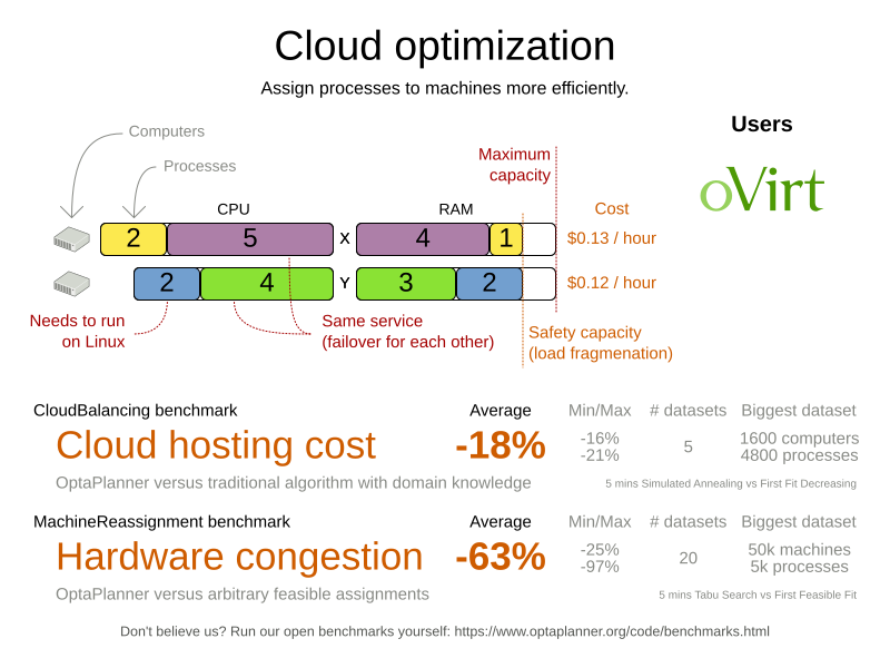
3.3.1.2. Problem size
| Problem Size | Computers | Processes | Search Space |
|---|---|---|---|
2computers-6processes |
2 |
6 |
64 |
3computers-9processes |
3 |
9 |
10^4 |
4computers-12processes |
4 |
12 |
10^7 |
100computers-300processes |
100 |
300 |
10^600 |
200computers-600processes |
200 |
600 |
10^1380 |
400computers-1200processes |
400 |
1200 |
10^3122 |
800computers-2400processes |
800 |
2400 |
10^6967 |
3.3.2. Using the domain model
3.3.2.1. Domain model design
Using a domain model helps determine which classes are planning entities and which of their properties are planning variables. It also helps to simplify constraints, improve performance, and increase flexibility for future needs.
To create a domain model, define all the objects that represent the input data for the problem. In this simple example, the objects are processes and computers.
A separate object in the domain model must represent a full data set of problem, which contains the input data as well as a solution. In this example, this object holds a list of computers and a list of processes. Each process is assigned to a computer; the distribution of processes between computers is the solution.
-
Draw a class diagram of your domain model.
-
Normalize it to remove duplicate data.
-
Write down some sample instances for each class.
-
Computer: represents a computer with certain hardware and maintenance costs.In this example, the sample instances for the
Computerclass are:cpuPower,memory,networkBandwidth,cost. -
Process: represents a process with a demand. Needs to be assigned to aComputerby OptaPlanner.Sample instances for
Processare:requiredCpuPower,requiredMemory, andrequiredNetworkBandwidth. -
CloudBalance: represents a problem. Contains everyComputerandProcessfor a certain data set.For an object representing the full data set and solution, a sample instance holding the score must be present. OptaPlanner can calculate and compare the scores for different solutions; the solution with the highest score is the optimal solution. Therefore, the sample instance for
CloudBalanceisscore.
-
-
Determine which relationships (or fields) change during planning.
-
Planning entity: The class (or classes) that OptaPlanner can change during solving. In this example, it is the class
Process, because OptaPlanner can assign processes to computers. -
Problem fact: A class representing input data that OptaPlanner cannot change.
-
Planning variable: The property (or properties) of a planning entity class that changes during solving. In this example, it is the property
computeron the classProcess. -
Planning solution: The class that represents a solution to the problem. This class must represent the full data set and contain all planning entities. In this example that is the class
CloudBalance.
-
In the UML class diagram below, the OptaPlanner concepts are already annotated:
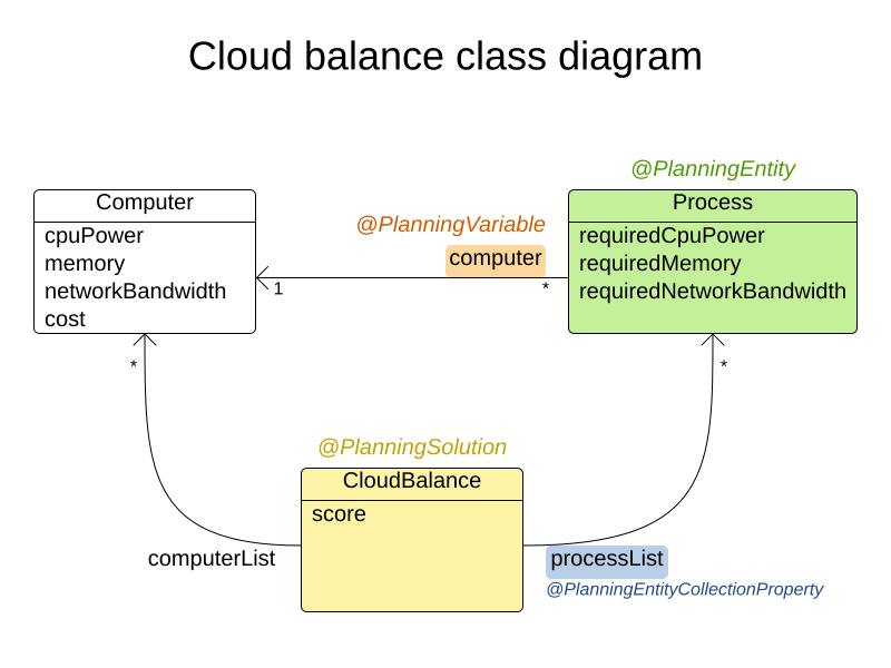
3.3.2.2. Domain model implementation
3.3.2.2.1. The Computer class
The Computer class is a POJO (Plain Old Java Object). Usually, you will have more of this kind of classes with input data.
public class CloudComputer ... {

    private int cpuPower;
    private int memory;
    private int networkBandwidth;
    private int cost;

    ... // getters
}
3.3.2.2.2. The Process class
The Process class is particularly important. It is the class that is modified during solving.
We need to tell OptaPlanner that it can change the property computer. To do this:
. Annotate the class with @PlanningEntity.
. Annotate the getter getComputer() with @PlanningVariable.
Of course, the property computer needs a setter too, so OptaPlanner can change it during solving.
@PlanningEntity(...)
public class CloudProcess ... {

    private int requiredCpuPower;
    private int requiredMemory;
    private int requiredNetworkBandwidth;

    private CloudComputer computer;

    ... // getters

    @PlanningVariable
    public CloudComputer getComputer() {
        return computer;
    }

    public void setComputer(CloudComputer computer) {
        computer = computer;
    }

    // ************************************************************************
    // Complex methods
    // ************************************************************************

    ...

}-
OptaPlanner needs to know which values it can choose from to assign to the property
computer. Those values are retrieved from the methodCloudBalance.getComputerList()on the planning solution, which returns a list of all computers in the current data set. -
The
@PlanningVariableautomatically matches with the@ValueRangeProvideronCloudBalance.getComputerList().
|
Instead of getter annotations, it is also possible to use field annotations. |
3.3.2.2.3. The CloudBalance class
The CloudBalance class has a @PlanningSolution annotation.
-
It holds a list of all computers and a list of all processes.
-
It represents both the planning problem and (if it is initialized) the planning solution.
-
To save a solution, OptaPlanner initializes a new instance of the class.
-
The
processListproperty holds a list of processes. OptaPlanner can change the processes, allocating them to different computers. Therefore, a process is a planning entity and the list of processes is a collection of planning entities. We annotate the gettergetProcessList()with@PlanningEntityCollectionProperty. -
The
computerListproperty holds a list of computers. OptaPlanner cannot change the computers. Therefore, a computer is a problem fact. Especially for Constraint Streams, the propertycomputerListneeds to be annotated with a@ProblemFactCollectionPropertyso that OptaPlanner can retrieve the list of computers (problem facts) and make it available to the rule engine. -
The
CloudBalanceclass also has a@PlanningScoreannotated propertyscore, which is theScoreof that solution in its current state. OptaPlanner automatically updates it when it calculates aScorefor a solution instance. Therefore, this property needs a setter.
-
@PlanningSolution
public class CloudBalance ... {

    private List<CloudComputer> computerList;

    private List<CloudProcess> processList;

    private HardSoftScore score;

    @ValueRangeProvider
    @ProblemFactCollectionProperty
    public List<CloudComputer> getComputerList() {
        return computerList;
    }

    @PlanningEntityCollectionProperty
    public List<CloudProcess> getProcessList() {
        return processList;
    }

    @PlanningScore
    public HardSoftScore getScore() {
        return score;
    }

    public void setScore(HardSoftScore score) {
        this.score = score;
    }

    ...
}
3.3.3. Run the cloud balancing Hello World
-
Create a run configuration with the following main class:
org.optaplanner.examples.cloudbalancing.app.CloudBalancingHelloWorldBy default, the Cloud Balancing Hello World is configured to run for 120 seconds.
It executes the following code:
public class CloudBalancingHelloWorld {

    public static void main(String[] args) {
        // Build the Solver
        SolverFactory<CloudBalance> solverFactory = SolverFactory.createFromXmlResource(
                "org/optaplanner/examples/cloudbalancing/solver/cloudBalancingSolverConfig.xml");
        Solver<CloudBalance> solver = solverFactory.buildSolver();

        // Load a problem with 400 computers and 1200 processes
        CloudBalance unsolvedCloudBalance = new CloudBalancingGenerator().createCloudBalance(400, 1200);

        // Solve the problem
        CloudBalance solvedCloudBalance = solver.solve(unsolvedCloudBalance);

        // Display the result
        System.out.println("\nSolved cloudBalance with 400 computers and 1200 processes:\n"
                + toDisplayString(solvedCloudBalance));
    }

    ...
}
The code example does the following:
-
Build the
Solverbased on a solver configuration which can come from an XML file as classpath resource:SolverFactory<CloudBalance> solverFactory = SolverFactory.createFromXmlResource( "org/optaplanner/examples/cloudbalancing/solver/cloudBalancingSolverConfig.xml"); Solver<CloudBalance> solver = solverFactory.buildSolver();Or to avoid XML, build it through the programmatic API instead:
        SolverFactory<CloudBalance> solverFactory = SolverFactory.create(new SolverConfig()
                .withSolutionClass(CloudBalance.class)
                .withEntityClasses(CloudProcess.class)
                .withEasyScoreCalculatorClass(CloudBalancingEasyScoreCalculator.class)
                .withTerminationSpentLimit(Duration.ofMinutes(2)));
        Solver<CloudBalance> solver = solverFactory.buildSolver();
The solver configuration is explained in the next section.
-
Load the problem.
CloudBalancingGeneratorgenerates a random problem: replace this with a class that loads a real problem, for example from a database.CloudBalance unsolvedCloudBalance = new CloudBalancingGenerator().createCloudBalance(400, 1200); -
Solve the problem.
CloudBalance solvedCloudBalance = solver.solve(unsolvedCloudBalance); -
Display the result.
        System.out.println("\nSolved cloudBalance with 400 computers and 1200 processes:\n"
                + toDisplayString(solvedCloudBalance));
3.3.4. Solver configuration
The solver configuration file determines how the solving process works; it is considered a part of the code.
The file is named cloudBalancingSolverConfig.xml.
<?xml version="1.0" encoding="UTF-8"?>
<solver xmlns="https://www.optaplanner.org/xsd/solver" xmlns:xsi="http://www.w3.org/2001/XMLSchema-instance"
    xsi:schemaLocation="https://www.optaplanner.org/xsd/solver https://www.optaplanner.org/xsd/solver/solver.xsd">
  <!-- Domain model configuration -->
  <solutionClass>org.optaplanner.examples.cloudbalancing.domain.CloudBalance</solutionClass>
  <entityClass>org.optaplanner.examples.cloudbalancing.domain.CloudProcess</entityClass>

  <!-- Score configuration -->
  <scoreDirectorFactory>
    <easyScoreCalculatorClass>org.optaplanner.examples.cloudbalancing.optional.score.CloudBalancingEasyScoreCalculator</easyScoreCalculatorClass>
    <!--<constraintProviderClass>org.optaplanner.examples.cloudbalancing.score.CloudBalancingConstraintProvider</constraintProviderClass>-->
  </scoreDirectorFactory>

  <!-- Optimization algorithms configuration -->
  <termination>
    <secondsSpentLimit>30</secondsSpentLimit>
  </termination>
</solver>
This solver configuration consists of three parts:
-
Domain model configuration: What can OptaPlanner change?
We need to make OptaPlanner aware of our domain classes, annotated with
@PlanningEntityand@PlanningSolutionannotations:<solutionClass>org.optaplanner.examples.cloudbalancing.domain.CloudBalance</solutionClass> <entityClass>org.optaplanner.examples.cloudbalancing.domain.CloudProcess</entityClass> -
Score configuration: How should OptaPlanner optimize the planning variables? What is our goal?
Since we have hard and soft constraints, we use a
HardSoftScore. But we need to tell OptaPlanner how to calculate the score, depending on our business requirements. Further down, we will look into two alternatives to calculate the score, such as using an easy Java implementation, or Constraint Streams.<scoreDirectorFactory> <easyScoreCalculatorClass>org.optaplanner.examples.cloudbalancing.optional.score.CloudBalancingEasyScoreCalculator</easyScoreCalculatorClass> <!--<constraintProviderClass>org.optaplanner.examples.cloudbalancing.score.CloudBalancingConstraintProvider</constraintProviderClass>--> </scoreDirectorFactory> -
Optimization algorithms configuration: How should OptaPlanner optimize it?
In this case, we use the default optimization algorithms (because no explicit optimization algorithms are configured) for 30 seconds:
  <termination>
    <secondsSpentLimit>30</secondsSpentLimit>
  </termination>
OptaPlanner should get a good result in seconds (and even in less than 15 milliseconds with real-time planning), but the more time it has, the better the results. Advanced use cases might use different termination criteria than a hard time limit.
The default algorithms already easily surpass human planners and most in-house implementations. Use the Benchmarker to power tweak to get even better results.
3.3.5. Score configuration
OptaPlanner searches for the solution with the highest Score.
This example uses a HardSoftScore, which means OptaPlanner looks for the solution with no hard constraints broken (fulfill hardware requirements) and as little as possible soft constraints broken (minimize maintenance cost).
Of course, OptaPlanner needs to be told about these domain-specific score constraints. There are several ways to implement such a score function:
3.3.5.1. Easy Java score configuration
One way to define a score function is to implement the interface EasyScoreCalculator in plain Java.
  <scoreDirectorFactory>
    <easyScoreCalculatorClass>org.optaplanner.examples.cloudbalancing.optional.score.CloudBalancingEasyScoreCalculator</easyScoreCalculatorClass>
  </scoreDirectorFactory>
Just implement the calculateScore(Solution) method to return a HardSoftScore instance.
public class CloudBalancingEasyScoreCalculator
    implements EasyScoreCalculator<CloudBalance, HardSoftScore> {

    /**
     * A very simple implementation. The double loop can easily be removed by using Maps as shown in
     * {@link CloudBalancingMapBasedEasyScoreCalculator#calculateScore(CloudBalance)}.
     */
    @Override
    public HardSoftScore calculateScore(CloudBalance cloudBalance) {
        int hardScore = 0;
        int softScore = 0;
        for (CloudComputer computer : cloudBalance.getComputerList()) {
            int cpuPowerUsage = 0;
            int memoryUsage = 0;
            int networkBandwidthUsage = 0;
            boolean used = false;

            // Calculate usage
            for (CloudProcess process : cloudBalance.getProcessList()) {
                if (computer.equals(process.getComputer())) {
                    cpuPowerUsage += process.getRequiredCpuPower();
                    memoryUsage += process.getRequiredMemory();
                    networkBandwidthUsage += process.getRequiredNetworkBandwidth();
                    used = true;
                }
            }

            // Hard constraints
            int cpuPowerAvailable = computer.getCpuPower() - cpuPowerUsage;
            if (cpuPowerAvailable < 0) {
                hardScore += cpuPowerAvailable;
            }
            int memoryAvailable = computer.getMemory() - memoryUsage;
            if (memoryAvailable < 0) {
                hardScore += memoryAvailable;
            }
            int networkBandwidthAvailable = computer.getNetworkBandwidth() - networkBandwidthUsage;
            if (networkBandwidthAvailable < 0) {
                hardScore += networkBandwidthAvailable;
            }

            // Soft constraints
            if (used) {
                softScore -= computer.getCost();
            }
        }
        return HardSoftScore.of(hardScore, softScore);
    }

}
Even if we optimize the code above to use Maps to iterate through the processList only once, it is still slow because it does not do incremental score calculation.
To fix that, either use constraint streams, incremental Java score calculation or Drools score calculation.
3.3.5.2. Constraint streams score configuration
Constraint Streams use incremental calculation.
To use it, implement the interface ConstraintProvider in Java.
  <scoreDirectorFactory>
    <constraintProviderClass>org.optaplanner.examples.cloudbalancing.score.CloudBalancingConstraintProvider</constraintProviderClass>
  </scoreDirectorFactory>
We want to make sure that all computers have enough CPU, RAM and network bandwidth to support all their processes, so we make these hard constraints. If those constraints are met, we want to minimize the maintenance cost, so we add that as a soft constraint.
public class CloudBalancingConstraintProvider implements ConstraintProvider {

    @Override
    public Constraint[] defineConstraints(ConstraintFactory constraintFactory) {
        return new Constraint[] {
                requiredCpuPowerTotal(constraintFactory),
                requiredMemoryTotal(constraintFactory),
                requiredNetworkBandwidthTotal(constraintFactory),
                computerCost(constraintFactory)
        };
    }

    Constraint requiredCpuPowerTotal(ConstraintFactory constraintFactory) {
        return constraintFactory.forEach(CloudProcess.class)
                .groupBy(CloudProcess::getComputer, sum(CloudProcess::getRequiredCpuPower))
                .filter((computer, requiredCpuPower) -> requiredCpuPower > computer.getCpuPower())
                .penalize(HardSoftScore.ONE_HARD,
                        (computer, requiredCpuPower) -> requiredCpuPower - computer.getCpuPower())
                .asConstraint("requiredCpuPowerTotal");
    }

    Constraint requiredMemoryTotal(ConstraintFactory constraintFactory) {
        return constraintFactory.forEach(CloudProcess.class)
                .groupBy(CloudProcess::getComputer, sum(CloudProcess::getRequiredMemory))
                .filter((computer, requiredMemory) -> requiredMemory > computer.getMemory())
                .penalize(HardSoftScore.ONE_HARD,
                        (computer, requiredMemory) -> requiredMemory - computer.getMemory())
                .asConstraint("requiredMemoryTotal");
    }

    Constraint requiredNetworkBandwidthTotal(ConstraintFactory constraintFactory) {
        return constraintFactory.forEach(CloudProcess.class)
                .groupBy(CloudProcess::getComputer, sum(CloudProcess::getRequiredNetworkBandwidth))
                .filter((computer, requiredNetworkBandwidth) -> requiredNetworkBandwidth > computer.getNetworkBandwidth())
                .penalize(HardSoftScore.ONE_HARD,
                        (computer, requiredNetworkBandwidth) -> requiredNetworkBandwidth - computer.getNetworkBandwidth())
                .asConstraint("requiredNetworkBandwidthTotal");
    }

    Constraint computerCost(ConstraintFactory constraintFactory) {
        return constraintFactory.forEach(CloudComputer.class)
                .ifExists(CloudProcess.class, equal(Function.identity(), CloudProcess::getComputer))
                .penalize(HardSoftScore.ONE_SOFT,
                        CloudComputer::getCost)
                .asConstraint("computerCost");
    }

}
3.3.5.3. Incremental Java score configuration
Another way to define a score function is to implement the interface IncrementalScoreCalculator in plain Java.
  <scoreDirectorFactory>
    <easyScoreCalculatorClass>org.optaplanner.examples.cloudbalancing.optional.score.CloudBalancingIncrementalScoreCalculator</easyScoreCalculatorClass>
</scoreDirectorFactory>public class CloudBalancingIncrementalScoreCalculator
implements IncrementalScoreCalculator<CloudBalance, HardSoftScore> {
private Map<CloudComputer, Integer> cpuPowerUsageMap;
private Map<CloudComputer, Integer> memoryUsageMap;
private Map<CloudComputer, Integer> networkBandwidthUsageMap;
private Map<CloudComputer, Integer> processCountMap;
private int hardScore;
private int softScore;
@Override
public void resetWorkingSolution(CloudBalance cloudBalance) {
int computerListSize = cloudBalance.getComputerList().size();
cpuPowerUsageMap = new HashMap<>(computerListSize);
memoryUsageMap = new HashMap<>(computerListSize);
networkBandwidthUsageMap = new HashMap<>(computerListSize);
processCountMap = new HashMap<>(computerListSize);
for (CloudComputer computer : cloudBalance.getComputerList()) {
cpuPowerUsageMap.put(computer, 0);
memoryUsageMap.put(computer, 0);
networkBandwidthUsageMap.put(computer, 0);
processCountMap.put(computer, 0);
}
hardScore = 0;
softScore = 0;
for (CloudProcess process : cloudBalance.getProcessList()) {
insert(process);
}
}
@Override
public void beforeVariableChanged(Object entity, String variableName) {
retract((CloudProcess) entity);
}
@Override
public void afterVariableChanged(Object entity, String variableName) {
insert((CloudProcess) entity);
}
@Override
public void beforeEntityRemoved(Object entity) {
retract((CloudProcess) entity);
}
...
private void insert(CloudProcess process) {
CloudComputer computer = process.getComputer();
if (computer != null) {
int cpuPower = computer.getCpuPower();
int oldCpuPowerUsage = cpuPowerUsageMap.get(computer);
int oldCpuPowerAvailable = cpuPower - oldCpuPowerUsage;
int newCpuPowerUsage = oldCpuPowerUsage + process.getRequiredCpuPower();
int newCpuPowerAvailable = cpuPower - newCpuPowerUsage;
hardScore += Math.min(newCpuPowerAvailable, 0) - Math.min(oldCpuPowerAvailable, 0);
cpuPowerUsageMap.put(computer, newCpuPowerUsage);
int memory = computer.getMemory();
int oldMemoryUsage = memoryUsageMap.get(computer);
int oldMemoryAvailable = memory - oldMemoryUsage;
int newMemoryUsage = oldMemoryUsage + process.getRequiredMemory();
int newMemoryAvailable = memory - newMemoryUsage;
hardScore += Math.min(newMemoryAvailable, 0) - Math.min(oldMemoryAvailable, 0);
memoryUsageMap.put(computer, newMemoryUsage);
int networkBandwidth = computer.getNetworkBandwidth();
int oldNetworkBandwidthUsage = networkBandwidthUsageMap.get(computer);
int oldNetworkBandwidthAvailable = networkBandwidth - oldNetworkBandwidthUsage;
int newNetworkBandwidthUsage = oldNetworkBandwidthUsage + process.getRequiredNetworkBandwidth();
int newNetworkBandwidthAvailable = networkBandwidth - newNetworkBandwidthUsage;
hardScore += Math.min(newNetworkBandwidthAvailable, 0) - Math.min(oldNetworkBandwidthAvailable, 0);
networkBandwidthUsageMap.put(computer, newNetworkBandwidthUsage);
int oldProcessCount = processCountMap.get(computer);
if (oldProcessCount == 0) {
softScore -= computer.getCost();
}
int newProcessCount = oldProcessCount + 1;
processCountMap.put(computer, newProcessCount);
}
}
private void retract(CloudProcess process) {
CloudComputer computer = process.getComputer();
if (computer != null) {
int cpuPower = computer.getCpuPower();
int oldCpuPowerUsage = cpuPowerUsageMap.get(computer);
int oldCpuPowerAvailable = cpuPower - oldCpuPowerUsage;
int newCpuPowerUsage = oldCpuPowerUsage - process.getRequiredCpuPower();
int newCpuPowerAvailable = cpuPower - newCpuPowerUsage;
hardScore += Math.min(newCpuPowerAvailable, 0) - Math.min(oldCpuPowerAvailable, 0);
cpuPowerUsageMap.put(computer, newCpuPowerUsage);
int memory = computer.getMemory();
int oldMemoryUsage = memoryUsageMap.get(computer);
int oldMemoryAvailable = memory - oldMemoryUsage;
int newMemoryUsage = oldMemoryUsage - process.getRequiredMemory();
int newMemoryAvailable = memory - newMemoryUsage;
hardScore += Math.min(newMemoryAvailable, 0) - Math.min(oldMemoryAvailable, 0);
memoryUsageMap.put(computer, newMemoryUsage);
int networkBandwidth = computer.getNetworkBandwidth();
int oldNetworkBandwidthUsage = networkBandwidthUsageMap.get(computer);
int oldNetworkBandwidthAvailable = networkBandwidth - oldNetworkBandwidthUsage;
int newNetworkBandwidthUsage = oldNetworkBandwidthUsage - process.getRequiredNetworkBandwidth();
int newNetworkBandwidthAvailable = networkBandwidth - newNetworkBandwidthUsage;
hardScore += Math.min(newNetworkBandwidthAvailable, 0) - Math.min(oldNetworkBandwidthAvailable, 0);
networkBandwidthUsageMap.put(computer, newNetworkBandwidthUsage);
int oldProcessCount = processCountMap.get(computer);
int newProcessCount = oldProcessCount - 1;
if (newProcessCount == 0) {
softScore += computer.getCost();
}
processCountMap.put(computer, newProcessCount);
}
}
@Override
public HardSoftScore calculateScore() {
return HardSoftScore.of(hardScore, softScore);
}
}This score calculation is the fastest we can possibly make it. It reacts to every planning variable change, making the smallest possible adjustment to the score.
3.3.6. Beyond this tutorial
Now that this simple example works, you can try going further. For example, you can enrich the domain model and add extra constraints such as these:
-
Each
Processbelongs to aService. A computer might crash, so processes running the same service must be assigned to different computers. -
Each
Computeris located in aBuilding. A building might burn down, so processes of the same services should (or must) be assigned to computers in different buildings.
3.4. Traveling salesman (TSP - traveling salesman problem)
3.4.1. Problem description
Given a list of cities, find the shortest tour for a salesman that visits each city exactly once.
The problem is defined by Wikipedia. It is one of the most intensively studied problems in computational mathematics. Yet, in the real world, it is often only part of a planning problem, along with other constraints, such as employee shift rostering constraints.
3.4.2. Problem size
dj38     has  38 cities with a search space of   10^43.
europe40 has  40 cities with a search space of   10^46.
st70     has  70 cities with a search space of   10^98.
pcb442   has 442 cities with a search space of  10^976.
lu980    has 980 cities with a search space of 10^2504.
3.4.3. Problem difficulty
Despite TSP’s simple definition, the problem is surprisingly hard to solve. Because it is an NP-hard problem (like most planning problems), the optimal solution for a specific problem dataset can change a lot when that problem dataset is slightly altered:
3.5. Tennis club scheduling
3.5.1. Problem description
Every week the tennis club has four teams playing round robin against each other. Assign those four spots to the teams fairly.
Hard constraints:
-
Conflict: A team can only play once per day.
-
Unavailability: Some teams are unavailable on some dates.
Medium constraints:
-
Fair assignment: All teams should play an (almost) equal number of times.
Soft constraints:
-
Evenly confrontation: Each team should play against every other team an equal number of times.
3.5.2. Problem size
munich-7teams has 7 teams, 18 days, 12 unavailabilityPenalties and 72 teamAssignments with a search space of 10^60.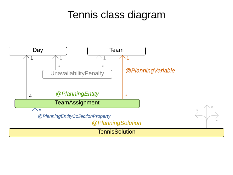
3.6. Meeting scheduling
3.6.1. Problem description
Assign each meeting to a starting time and a room. Meetings have different durations.
Hard constraints:
-
Room conflict: two meetings must not use the same room at the same time.
-
Required attendance: A person cannot have two required meetings at the same time.
-
Required room capacity: A meeting must not be in a room that doesn’t fit all of the meeting’s attendees.
-
Start and end on same day: A meeting shouldn’t be scheduled over multiple days.
Medium constraints:
-
Preferred attendance: A person cannot have two preferred meetings at the same time, nor a preferred and a required meeting at the same time.
Soft constraints:
-
Sooner rather than later: Schedule all meetings as soon as possible.
-
A break between meetings: Any two meetings should have at least one time grain break between them.
-
Overlapping meetings: To minimize the number of meetings in parallel so people don’t have to choose one meeting over the other.
-
Assign larger rooms first: If a larger room is available any meeting should be assigned to that room in order to accommodate as many people as possible even if they haven’t signed up to that meeting.
-
Room stability: If a person has two consecutive meetings with two or less time grains break between them they better be in the same room.
3.6.2. Problem size
50meetings-160timegrains-5rooms  has  50 meetings, 160 timeGrains and 5 rooms with a search space of 10^145.
100meetings-320timegrains-5rooms has 100 meetings, 320 timeGrains and 5 rooms with a search space of 10^320.
200meetings-640timegrains-5rooms has 200 meetings, 640 timeGrains and 5 rooms with a search space of 10^701.
400meetings-1280timegrains-5rooms has 400 meetings, 1280 timeGrains and 5 rooms with a search space of 10^1522.
800meetings-2560timegrains-5rooms has 800 meetings, 2560 timeGrains and 5 rooms with a search space of 10^3285.
3.7. Course timetabling (ITC 2007 Track 3 - Curriculum Course Scheduling)
3.7.1. Problem description
Schedule each lecture into a timeslot and into a room.
Hard constraints:
-
Teacher conflict: A teacher must not have two lectures in the same period.
-
Curriculum conflict: A curriculum must not have two lectures in the same period.
-
Room occupancy: two lectures must not be in the same room in the same period.
-
Unavailable period (specified per dataset): A specific lecture must not be assigned to a specific period.
Soft constraints:
-
Room capacity: A room’s capacity should not be less than the number of students in its lecture.
-
Minimum working days: Lectures of the same course should be spread out into a minimum number of days.
-
Curriculum compactness: Lectures belonging to the same curriculum should be adjacent to each other (so in consecutive periods).
-
Room stability: Lectures of the same course should be assigned to the same room.
The problem is defined by the International Timetabling Competition 2007 track 3.
3.7.2. Problem size
comp01 has 24 teachers,  14 curricula,  30 courses, 160 lectures, 30 periods,  6 rooms and   53 unavailable period constraints with a search space of  10^360.
comp02 has 71 teachers,  70 curricula,  82 courses, 283 lectures, 25 periods, 16 rooms and  513 unavailable period constraints with a search space of  10^736.
comp03 has 61 teachers,  68 curricula,  72 courses, 251 lectures, 25 periods, 16 rooms and  382 unavailable period constraints with a search space of  10^653.
comp04 has 70 teachers,  57 curricula,  79 courses, 286 lectures, 25 periods, 18 rooms and  396 unavailable period constraints with a search space of  10^758.
comp05 has 47 teachers, 139 curricula,  54 courses, 152 lectures, 36 periods,  9 rooms and  771 unavailable period constraints with a search space of  10^381.
comp06 has 87 teachers,  70 curricula, 108 courses, 361 lectures, 25 periods, 18 rooms and  632 unavailable period constraints with a search space of  10^957.
comp07 has 99 teachers,  77 curricula, 131 courses, 434 lectures, 25 periods, 20 rooms and  667 unavailable period constraints with a search space of 10^1171.
comp08 has 76 teachers,  61 curricula,  86 courses, 324 lectures, 25 periods, 18 rooms and  478 unavailable period constraints with a search space of  10^859.
comp09 has 68 teachers,  75 curricula,  76 courses, 279 lectures, 25 periods, 18 rooms and  405 unavailable period constraints with a search space of  10^740.
comp10 has 88 teachers,  67 curricula, 115 courses, 370 lectures, 25 periods, 18 rooms and  694 unavailable period constraints with a search space of  10^981.
comp11 has 24 teachers,  13 curricula,  30 courses, 162 lectures, 45 periods,  5 rooms and   94 unavailable period constraints with a search space of  10^381.
comp12 has 74 teachers, 150 curricula,  88 courses, 218 lectures, 36 periods, 11 rooms and 1368 unavailable period constraints with a search space of  10^566.
comp13 has 77 teachers,  66 curricula,  82 courses, 308 lectures, 25 periods, 19 rooms and  468 unavailable period constraints with a search space of  10^824.
comp14 has 68 teachers,  60 curricula,  85 courses, 275 lectures, 25 periods, 17 rooms and  486 unavailable period constraints with a search space of  10^722.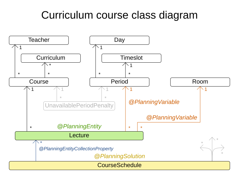
3.8. Machine reassignment (Google ROADEF 2012)
3.8.1. Problem description
Assign each process to a machine. All processes already have an original (unoptimized) assignment. Each process requires an amount of each resource (such as CPU, RAM, …). This is a more complex version of the Cloud Balancing example.
Hard constraints:
-
Maximum capacity: The maximum capacity for each resource for each machine must not be exceeded.
-
Conflict: Processes of the same service must run on distinct machines.
-
Spread: Processes of the same service must be spread out across locations.
-
Dependency: The processes of a service depending on another service must run in the neighborhood of a process of the other service.
-
Transient usage: Some resources are transient and count towards the maximum capacity of both the original machine as the newly assigned machine.
Soft constraints:
-
Load: The safety capacity for each resource for each machine should not be exceeded.
-
Balance: Leave room for future assignments by balancing the available resources on each machine.
-
Process move cost: A process has a move cost.
-
Service move cost: A service has a move cost.
-
Machine move cost: Moving a process from machine A to machine B has another A-B specific move cost.
The problem is defined by the Google ROADEF/EURO Challenge 2012.
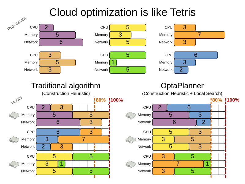
3.8.3. Problem size
model_a1_1 has  2 resources,  1 neighborhoods,   4 locations,    4 machines,    79 services,   100 processes and 1 balancePenalties with a search space of     10^60.
model_a1_2 has  4 resources,  2 neighborhoods,   4 locations,  100 machines,   980 services,  1000 processes and 0 balancePenalties with a search space of   10^2000.
model_a1_3 has  3 resources,  5 neighborhoods,  25 locations,  100 machines,   216 services,  1000 processes and 0 balancePenalties with a search space of   10^2000.
model_a1_4 has  3 resources, 50 neighborhoods,  50 locations,   50 machines,   142 services,  1000 processes and 1 balancePenalties with a search space of   10^1698.
model_a1_5 has  4 resources,  2 neighborhoods,   4 locations,   12 machines,   981 services,  1000 processes and 1 balancePenalties with a search space of   10^1079.
model_a2_1 has  3 resources,  1 neighborhoods,   1 locations,  100 machines,  1000 services,  1000 processes and 0 balancePenalties with a search space of   10^2000.
model_a2_2 has 12 resources,  5 neighborhoods,  25 locations,  100 machines,   170 services,  1000 processes and 0 balancePenalties with a search space of   10^2000.
model_a2_3 has 12 resources,  5 neighborhoods,  25 locations,  100 machines,   129 services,  1000 processes and 0 balancePenalties with a search space of   10^2000.
model_a2_4 has 12 resources,  5 neighborhoods,  25 locations,   50 machines,   180 services,  1000 processes and 1 balancePenalties with a search space of   10^1698.
model_a2_5 has 12 resources,  5 neighborhoods,  25 locations,   50 machines,   153 services,  1000 processes and 0 balancePenalties with a search space of   10^1698.
model_b_1  has 12 resources,  5 neighborhoods,  10 locations,  100 machines,  2512 services,  5000 processes and 0 balancePenalties with a search space of  10^10000.
model_b_2  has 12 resources,  5 neighborhoods,  10 locations,  100 machines,  2462 services,  5000 processes and 1 balancePenalties with a search space of  10^10000.
model_b_3  has  6 resources,  5 neighborhoods,  10 locations,  100 machines, 15025 services, 20000 processes and 0 balancePenalties with a search space of  10^40000.
model_b_4  has  6 resources,  5 neighborhoods,  50 locations,  500 machines,  1732 services, 20000 processes and 1 balancePenalties with a search space of  10^53979.
model_b_5  has  6 resources,  5 neighborhoods,  10 locations,  100 machines, 35082 services, 40000 processes and 0 balancePenalties with a search space of  10^80000.
model_b_6  has  6 resources,  5 neighborhoods,  50 locations,  200 machines, 14680 services, 40000 processes and 1 balancePenalties with a search space of  10^92041.
model_b_7  has  6 resources,  5 neighborhoods,  50 locations, 4000 machines, 15050 services, 40000 processes and 1 balancePenalties with a search space of 10^144082.
model_b_8  has  3 resources,  5 neighborhoods,  10 locations,  100 machines, 45030 services, 50000 processes and 0 balancePenalties with a search space of 10^100000.
model_b_9  has  3 resources,  5 neighborhoods, 100 locations, 1000 machines,  4609 services, 50000 processes and 1 balancePenalties with a search space of 10^150000.
model_b_10 has  3 resources,  5 neighborhoods, 100 locations, 5000 machines,  4896 services, 50000 processes and 1 balancePenalties with a search space of 10^184948.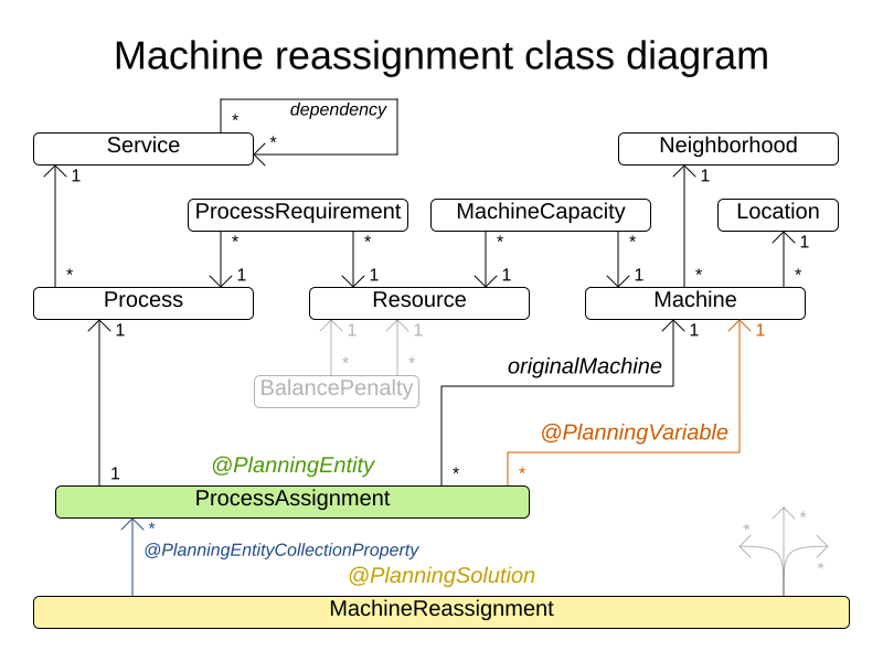
3.9. Vehicle routing
3.9.1. Problem description
Using a fleet of vehicles, pick up the objects of each customer and bring them to the depot. Each vehicle can service multiple customers, but it has a limited capacity.
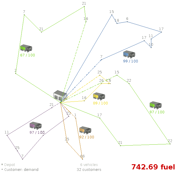
Besides the basic case (CVRP), there is also a variant with time windows (CVRPTW).
Hard constraints:
-
Vehicle capacity: a vehicle cannot carry more items then its capacity.
-
Time windows (only in CVRPTW):
-
Travel time: Traveling from one location to another takes time.
-
Customer service duration: a vehicle must stay at the customer for the length of the service duration.
-
Customer ready time: a vehicle may arrive before the customer’s ready time, but it must wait until the ready time before servicing.
-
Customer due time: a vehicle must arrive on time, before the customer’s due time.
-
Soft constraints:
-
Total distance: minimize the total distance driven (fuel consumption) of all vehicles.
The capacitated vehicle routing problem (CVRP) and its timewindowed variant (CVRPTW) are defined by the VRP web.
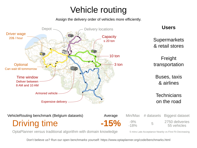
3.9.3. Problem size
CVRP instances (without time windows):
belgium-n50-k10             has  1 depots, 10 vehicles and   49 customers with a search space of   10^74.
belgium-n100-k10            has  1 depots, 10 vehicles and   99 customers with a search space of  10^170.
belgium-n500-k20            has  1 depots, 20 vehicles and  499 customers with a search space of 10^1168.
belgium-n1000-k20           has  1 depots, 20 vehicles and  999 customers with a search space of 10^2607.
belgium-n2750-k55           has  1 depots, 55 vehicles and 2749 customers with a search space of 10^8380.
belgium-road-km-n50-k10     has  1 depots, 10 vehicles and   49 customers with a search space of   10^74.
belgium-road-km-n100-k10    has  1 depots, 10 vehicles and   99 customers with a search space of  10^170.
belgium-road-km-n500-k20    has  1 depots, 20 vehicles and  499 customers with a search space of 10^1168.
belgium-road-km-n1000-k20   has  1 depots, 20 vehicles and  999 customers with a search space of 10^2607.
belgium-road-km-n2750-k55   has  1 depots, 55 vehicles and 2749 customers with a search space of 10^8380.
belgium-road-time-n50-k10   has  1 depots, 10 vehicles and   49 customers with a search space of   10^74.
belgium-road-time-n100-k10  has  1 depots, 10 vehicles and   99 customers with a search space of  10^170.
belgium-road-time-n500-k20  has  1 depots, 20 vehicles and  499 customers with a search space of 10^1168.
belgium-road-time-n1000-k20 has  1 depots, 20 vehicles and  999 customers with a search space of 10^2607.
belgium-road-time-n2750-k55 has  1 depots, 55 vehicles and 2749 customers with a search space of 10^8380.
belgium-d2-n50-k10          has  2 depots, 10 vehicles and   48 customers with a search space of   10^74.
belgium-d3-n100-k10         has  3 depots, 10 vehicles and   97 customers with a search space of  10^170.
belgium-d5-n500-k20         has  5 depots, 20 vehicles and  495 customers with a search space of 10^1168.
belgium-d8-n1000-k20        has  8 depots, 20 vehicles and  992 customers with a search space of 10^2607.
belgium-d10-n2750-k55       has 10 depots, 55 vehicles and 2740 customers with a search space of 10^8380.

A-n32-k5  has 1 depots,  5 vehicles and  31 customers with a search space of  10^40.
A-n33-k5  has 1 depots,  5 vehicles and  32 customers with a search space of  10^41.
A-n33-k6  has 1 depots,  6 vehicles and  32 customers with a search space of  10^42.
A-n34-k5  has 1 depots,  5 vehicles and  33 customers with a search space of  10^43.
A-n36-k5  has 1 depots,  5 vehicles and  35 customers with a search space of  10^46.
A-n37-k5  has 1 depots,  5 vehicles and  36 customers with a search space of  10^48.
A-n37-k6  has 1 depots,  6 vehicles and  36 customers with a search space of  10^49.
A-n38-k5  has 1 depots,  5 vehicles and  37 customers with a search space of  10^49.
A-n39-k5  has 1 depots,  5 vehicles and  38 customers with a search space of  10^51.
A-n39-k6  has 1 depots,  6 vehicles and  38 customers with a search space of  10^52.
A-n44-k7  has 1 depots,  7 vehicles and  43 customers with a search space of  10^61.
A-n45-k6  has 1 depots,  6 vehicles and  44 customers with a search space of  10^62.
A-n45-k7  has 1 depots,  7 vehicles and  44 customers with a search space of  10^63.
A-n46-k7  has 1 depots,  7 vehicles and  45 customers with a search space of  10^65.
A-n48-k7  has 1 depots,  7 vehicles and  47 customers with a search space of  10^68.
A-n53-k7  has 1 depots,  7 vehicles and  52 customers with a search space of  10^77.
A-n54-k7  has 1 depots,  7 vehicles and  53 customers with a search space of  10^79.
A-n55-k9  has 1 depots,  9 vehicles and  54 customers with a search space of  10^82.
A-n60-k9  has 1 depots,  9 vehicles and  59 customers with a search space of  10^91.
A-n61-k9  has 1 depots,  9 vehicles and  60 customers with a search space of  10^93.
A-n62-k8  has 1 depots,  8 vehicles and  61 customers with a search space of  10^94.
A-n63-k9  has 1 depots,  9 vehicles and  62 customers with a search space of  10^97.
A-n63-k10 has 1 depots, 10 vehicles and  62 customers with a search space of  10^98.
A-n64-k9  has 1 depots,  9 vehicles and  63 customers with a search space of  10^99.
A-n65-k9  has 1 depots,  9 vehicles and  64 customers with a search space of 10^101.
A-n69-k9  has 1 depots,  9 vehicles and  68 customers with a search space of 10^108.
A-n80-k10 has 1 depots, 10 vehicles and  79 customers with a search space of 10^130.
F-n45-k4  has 1 depots,  4 vehicles and  44 customers with a search space of  10^60.
F-n72-k4  has 1 depots,  4 vehicles and  71 customers with a search space of 10^108.
F-n135-k7 has 1 depots,  7 vehicles and 134 customers with a search space of 10^240.
CVRPTW instances (with time windows):
belgium-tw-d2-n50-k10    has  2 depots, 10 vehicles and   48 customers with a search space of   10^74.
belgium-tw-d3-n100-k10   has  3 depots, 10 vehicles and   97 customers with a search space of  10^170.
belgium-tw-d5-n500-k20   has  5 depots, 20 vehicles and  495 customers with a search space of 10^1168.
belgium-tw-d8-n1000-k20  has  8 depots, 20 vehicles and  992 customers with a search space of 10^2607.
belgium-tw-d10-n2750-k55 has 10 depots, 55 vehicles and 2740 customers with a search space of 10^8380.
belgium-tw-n50-k10       has  1 depots, 10 vehicles and   49 customers with a search space of   10^74.
belgium-tw-n100-k10      has  1 depots, 10 vehicles and   99 customers with a search space of  10^170.
belgium-tw-n500-k20      has  1 depots, 20 vehicles and  499 customers with a search space of 10^1168.
belgium-tw-n1000-k20     has  1 depots, 20 vehicles and  999 customers with a search space of 10^2607.
belgium-tw-n2750-k55     has  1 depots, 55 vehicles and 2749 customers with a search space of 10^8380.

Solomon_025_C101       has 1 depots,  25 vehicles and   25 customers with a search space of   10^40.
Solomon_025_C201       has 1 depots,  25 vehicles and   25 customers with a search space of   10^40.
Solomon_025_R101       has 1 depots,  25 vehicles and   25 customers with a search space of   10^40.
Solomon_025_R201       has 1 depots,  25 vehicles and   25 customers with a search space of   10^40.
Solomon_025_RC101      has 1 depots,  25 vehicles and   25 customers with a search space of   10^40.
Solomon_025_RC201      has 1 depots,  25 vehicles and   25 customers with a search space of   10^40.
Solomon_100_C101       has 1 depots,  25 vehicles and  100 customers with a search space of  10^185.
Solomon_100_C201       has 1 depots,  25 vehicles and  100 customers with a search space of  10^185.
Solomon_100_R101       has 1 depots,  25 vehicles and  100 customers with a search space of  10^185.
Solomon_100_R201       has 1 depots,  25 vehicles and  100 customers with a search space of  10^185.
Solomon_100_RC101      has 1 depots,  25 vehicles and  100 customers with a search space of  10^185.
Solomon_100_RC201      has 1 depots,  25 vehicles and  100 customers with a search space of  10^185.
Homberger_0200_C1_2_1  has 1 depots,  50 vehicles and  200 customers with a search space of  10^429.
Homberger_0200_C2_2_1  has 1 depots,  50 vehicles and  200 customers with a search space of  10^429.
Homberger_0200_R1_2_1  has 1 depots,  50 vehicles and  200 customers with a search space of  10^429.
Homberger_0200_R2_2_1  has 1 depots,  50 vehicles and  200 customers with a search space of  10^429.
Homberger_0200_RC1_2_1 has 1 depots,  50 vehicles and  200 customers with a search space of  10^429.
Homberger_0200_RC2_2_1 has 1 depots,  50 vehicles and  200 customers with a search space of  10^429.
Homberger_0400_C1_4_1  has 1 depots, 100 vehicles and  400 customers with a search space of  10^978.
Homberger_0400_C2_4_1  has 1 depots, 100 vehicles and  400 customers with a search space of  10^978.
Homberger_0400_R1_4_1  has 1 depots, 100 vehicles and  400 customers with a search space of  10^978.
Homberger_0400_R2_4_1  has 1 depots, 100 vehicles and  400 customers with a search space of  10^978.
Homberger_0400_RC1_4_1 has 1 depots, 100 vehicles and  400 customers with a search space of  10^978.
Homberger_0400_RC2_4_1 has 1 depots, 100 vehicles and  400 customers with a search space of  10^978.
Homberger_0600_C1_6_1  has 1 depots, 150 vehicles and  600 customers with a search space of 10^1571.
Homberger_0600_C2_6_1  has 1 depots, 150 vehicles and  600 customers with a search space of 10^1571.
Homberger_0600_R1_6_1  has 1 depots, 150 vehicles and  600 customers with a search space of 10^1571.
Homberger_0600_R2_6_1  has 1 depots, 150 vehicles and  600 customers with a search space of 10^1571.
Homberger_0600_RC1_6_1 has 1 depots, 150 vehicles and  600 customers with a search space of 10^1571.
Homberger_0600_RC2_6_1 has 1 depots, 150 vehicles and  600 customers with a search space of 10^1571.
Homberger_0800_C1_8_1  has 1 depots, 200 vehicles and  800 customers with a search space of 10^2195.
Homberger_0800_C2_8_1  has 1 depots, 200 vehicles and  800 customers with a search space of 10^2195.
Homberger_0800_R1_8_1  has 1 depots, 200 vehicles and  800 customers with a search space of 10^2195.
Homberger_0800_R2_8_1  has 1 depots, 200 vehicles and  800 customers with a search space of 10^2195.
Homberger_0800_RC1_8_1 has 1 depots, 200 vehicles and  800 customers with a search space of 10^2195.
Homberger_0800_RC2_8_1 has 1 depots, 200 vehicles and  800 customers with a search space of 10^2195.
Homberger_1000_C110_1  has 1 depots, 250 vehicles and 1000 customers with a search space of 10^2840.
Homberger_1000_C210_1  has 1 depots, 250 vehicles and 1000 customers with a search space of 10^2840.
Homberger_1000_R110_1  has 1 depots, 250 vehicles and 1000 customers with a search space of 10^2840.
Homberger_1000_R210_1  has 1 depots, 250 vehicles and 1000 customers with a search space of 10^2840.
Homberger_1000_RC110_1 has 1 depots, 250 vehicles and 1000 customers with a search space of 10^2840.
Homberger_1000_RC210_1 has 1 depots, 250 vehicles and 1000 customers with a search space of 10^2840.
3.9.4. Domain model
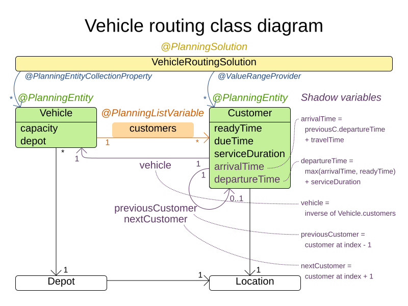
The vehicle routing with timewindows domain model makes heavily use of shadow variables.
This allows it to express its constraints more naturally, because properties such as arrivalTime and departureTime, are directly available on the domain model.
3.9.4.1. Road distances instead of air distances
In the real world, vehicles cannot follow a straight line from location to location: they have to use roads and highways. From a business point of view, this matters a lot:
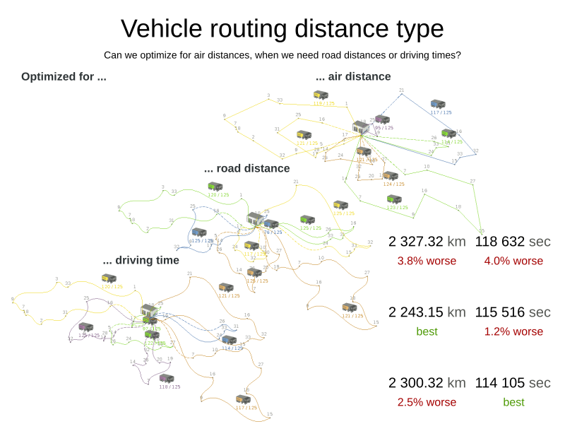
For the optimization algorithm, this does not matter much, as long as the distance between two points can be looked up (and are preferably precalculated). The road cost does not even need to be a distance, it can also be travel time, fuel cost, or a weighted function of those. There are several technologies available to precalculate road costs, such as GraphHopper (embeddable, offline Java engine), Open MapQuest (web service) and Google Maps Client API (web service).
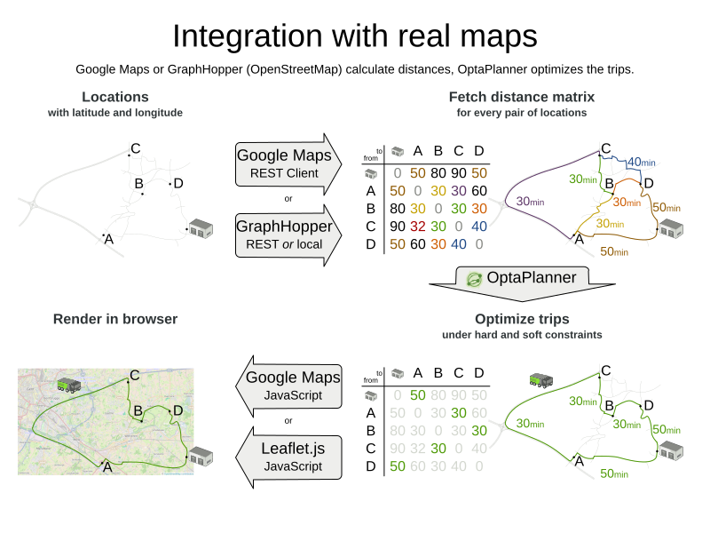
There are also several technologies to render it, such as Leaflet and Google Maps for developers:
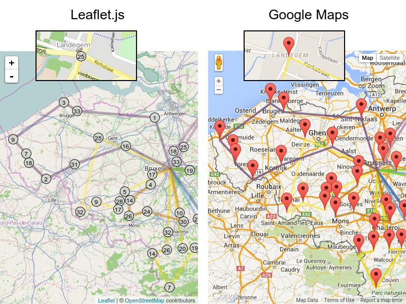
It is even possible to render the actual road routes with GraphHopper or Google Map Directions, but because of route overlaps on highways, it can become harder to see the standstill order:
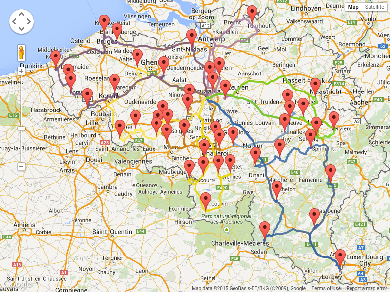
Take special care that the road costs between two points use the same optimization criteria as the one used in OptaPlanner. For example, GraphHopper etc will by default return the fastest route, not the shortest route. Don’t use the km (or miles) distances of the fastest GPS routes to optimize the shortest trip in OptaPlanner: this leads to a suboptimal solution as shown below:
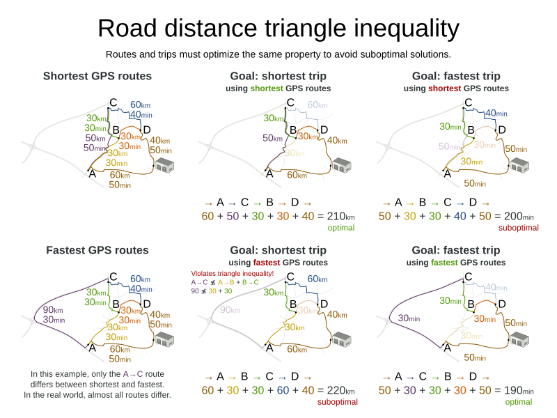
Contrary to popular belief, most users do not want the shortest route: they want the fastest route instead. They prefer highways over normal roads. They prefer normal roads over dirt roads. In the real world, the fastest and shortest route are rarely the same.
3.10. Project job scheduling
3.10.1. Problem description
Schedule all jobs in time and execution mode to minimize project delays. Each job is part of a project. A job can be executed in different ways: each way is an execution mode that implies a different duration but also different resource usages. This is a form of flexible job shop scheduling.
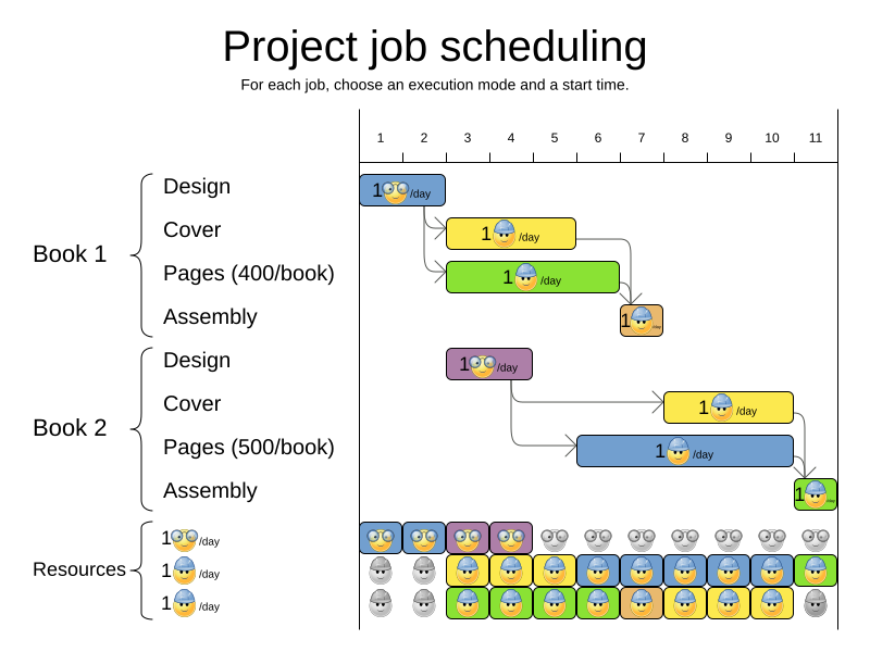
Hard constraints:
-
Job precedence: a job can only start when all its predecessor jobs are finished.
-
Resource capacity: do not use more resources than available.
-
Resources are local (shared between jobs of the same project) or global (shared between all jobs)
-
Resources are renewable (capacity available per day) or nonrenewable (capacity available for all days)
-
Medium constraints:
-
Total project delay: minimize the duration (makespan) of each project.
Soft constraints:
-
Total makespan: minimize the duration of the whole multi-project schedule.
The problem is defined by the MISTA 2013 challenge.
3.10.2. Problem size
Schedule A-1  has  2 projects,  24 jobs,   64 execution modes,  7 resources and  150 resource requirements.
Schedule A-2  has  2 projects,  44 jobs,  124 execution modes,  7 resources and  420 resource requirements.
Schedule A-3  has  2 projects,  64 jobs,  184 execution modes,  7 resources and  630 resource requirements.
Schedule A-4  has  5 projects,  60 jobs,  160 execution modes, 16 resources and  390 resource requirements.
Schedule A-5  has  5 projects, 110 jobs,  310 execution modes, 16 resources and  900 resource requirements.
Schedule A-6  has  5 projects, 160 jobs,  460 execution modes, 16 resources and 1440 resource requirements.
Schedule A-7  has 10 projects, 120 jobs,  320 execution modes, 22 resources and  900 resource requirements.
Schedule A-8  has 10 projects, 220 jobs,  620 execution modes, 22 resources and 1860 resource requirements.
Schedule A-9  has 10 projects, 320 jobs,  920 execution modes, 31 resources and 2880 resource requirements.
Schedule A-10 has 10 projects, 320 jobs,  920 execution modes, 31 resources and 2970 resource requirements.
Schedule B-1  has 10 projects, 120 jobs,  320 execution modes, 31 resources and  900 resource requirements.
Schedule B-2  has 10 projects, 220 jobs,  620 execution modes, 22 resources and 1740 resource requirements.
Schedule B-3  has 10 projects, 320 jobs,  920 execution modes, 31 resources and 3060 resource requirements.
Schedule B-4  has 15 projects, 180 jobs,  480 execution modes, 46 resources and 1530 resource requirements.
Schedule B-5  has 15 projects, 330 jobs,  930 execution modes, 46 resources and 2760 resource requirements.
Schedule B-6  has 15 projects, 480 jobs, 1380 execution modes, 46 resources and 4500 resource requirements.
Schedule B-7  has 20 projects, 240 jobs,  640 execution modes, 61 resources and 1710 resource requirements.
Schedule B-8  has 20 projects, 440 jobs, 1240 execution modes, 42 resources and 3180 resource requirements.
Schedule B-9  has 20 projects, 640 jobs, 1840 execution modes, 61 resources and 5940 resource requirements.
Schedule B-10 has 20 projects, 460 jobs, 1300 execution modes, 42 resources and 4260 resource requirements.
3.11. Hospital bed planning (PAS - Patient Admission Scheduling)
3.11.1. Problem description
Assign each patient (that will come to the hospital) into a bed for each night that the patient will stay in the hospital. Each bed belongs to a room and each room belongs to a department. The arrival and departure dates of the patients is fixed: only a bed needs to be assigned for each night.
This problem features overconstrained datasets.
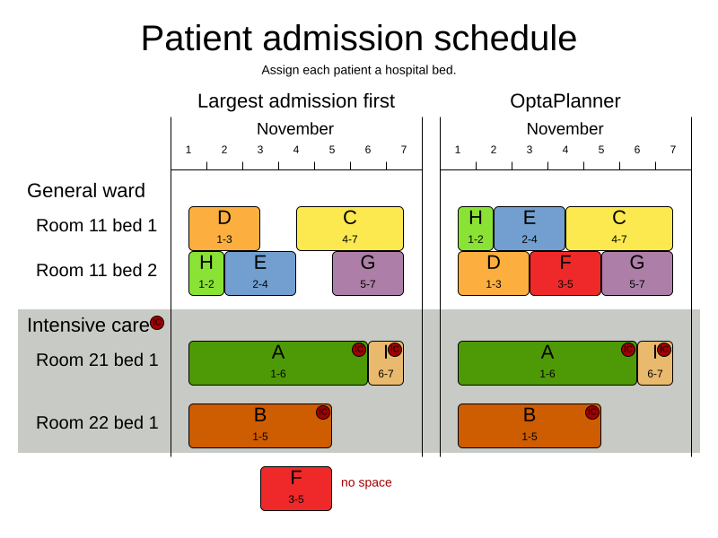
Hard constraints:
-
Two patients must not be assigned to the same bed in the same night. Weight:
-1000hard * conflictNightCount. -
A room can have a gender limitation: only females, only males, the same gender in the same night or no gender limitation at all. Weight:
-50hard * nightCount. -
A department can have a minimum or maximum age. Weight:
-100hard * nightCount. -
A patient can require a room with specific equipment(s). Weight:
-50hard * nightCount.
Medium constraints:
-
Assign every patient to a bed, unless the dataset is overconstrained. Weight:
-1medium * nightCount.
Soft constraints:
-
A patient can prefer a maximum room size, for example if he/she wants a single room. Weight:
-8soft * nightCount. -
A patient is best assigned to a department that specializes in his/her problem. Weight:
-10soft * nightCount. -
A patient is best assigned to a room that specializes in his/her problem. Weight:
-20soft * nightCount.-
That room speciality should be priority 1. Weight:
-10soft * (priority - 1) * nightCount.
-
-
A patient can prefer a room with specific equipment(s). Weight:
-20soft * nightCount.
The problem is a variant on Kaho’s Patient Scheduling and the datasets come from real world hospitals.
3.11.2. Problem size
overconstrained01 has 6 specialisms, 4 equipments, 1 departments,  25 rooms,  69 beds, 14 nights,  519 patients and  519 admissions with a search space of 10^958.
testdata01        has 4 specialisms, 2 equipments, 4 departments,  98 rooms, 286 beds, 14 nights,  652 patients and  652 admissions with a search space of 10^1603.
testdata02        has 6 specialisms, 2 equipments, 6 departments, 151 rooms, 465 beds, 14 nights,  755 patients and  755 admissions with a search space of 10^2015.
testdata03        has 5 specialisms, 2 equipments, 5 departments, 131 rooms, 395 beds, 14 nights,  708 patients and  708 admissions with a search space of 10^1840.
testdata04        has 6 specialisms, 2 equipments, 6 departments, 155 rooms, 471 beds, 14 nights,  746 patients and  746 admissions with a search space of 10^1995.
testdata05        has 4 specialisms, 2 equipments, 4 departments, 102 rooms, 325 beds, 14 nights,  587 patients and  587 admissions with a search space of 10^1476.
testdata06        has 4 specialisms, 2 equipments, 4 departments, 104 rooms, 313 beds, 14 nights,  685 patients and  685 admissions with a search space of 10^1711.
testdata07        has 6 specialisms, 4 equipments, 6 departments, 162 rooms, 472 beds, 14 nights,  519 patients and  519 admissions with a search space of 10^1389.
testdata08        has 6 specialisms, 4 equipments, 6 departments, 148 rooms, 441 beds, 21 nights,  895 patients and  895 admissions with a search space of 10^2368.
testdata09        has 4 specialisms, 4 equipments, 4 departments, 105 rooms, 310 beds, 28 nights, 1400 patients and 1400 admissions with a search space of 10^3490.
testdata10        has 4 specialisms, 4 equipments, 4 departments, 104 rooms, 308 beds, 56 nights, 1575 patients and 1575 admissions with a search space of 10^3922.
testdata11        has 4 specialisms, 4 equipments, 4 departments, 107 rooms, 318 beds, 91 nights, 2514 patients and 2514 admissions with a search space of 10^6295.
testdata12        has 4 specialisms, 4 equipments, 4 departments, 105 rooms, 310 beds, 84 nights, 2750 patients and 2750 admissions with a search space of 10^6856.
testdata13        has 5 specialisms, 4 equipments, 5 departments, 125 rooms, 368 beds, 28 nights,  907 patients and 1109 admissions with a search space of 10^2847.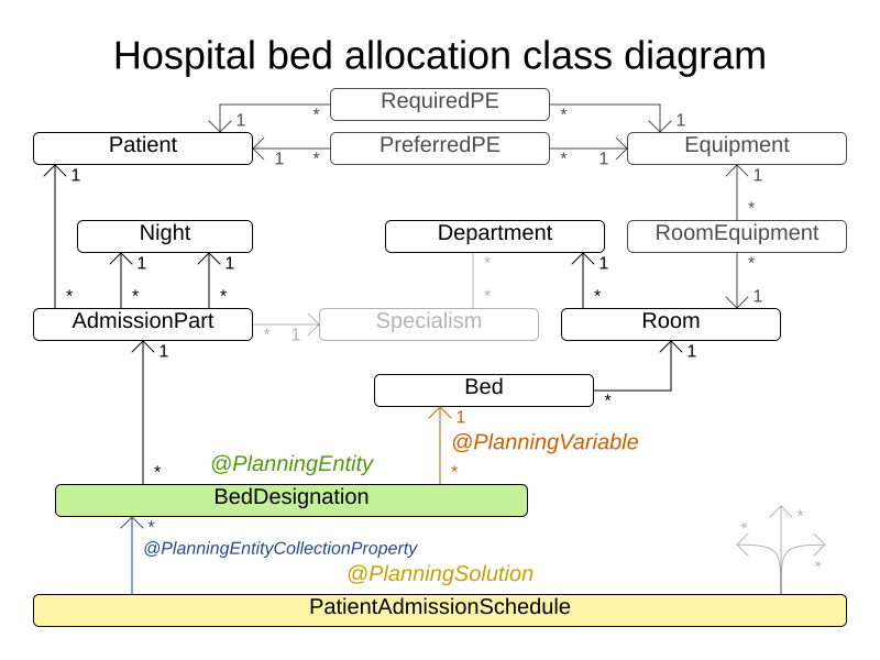
3.12. Task assigning
3.12.1. Problem description
Assign each task to a spot in an employee’s queue. Each task has a duration which is affected by the employee’s affinity level with the task’s customer.
Hard constraints:
-
Skill: Each task requires one or more skills. The employee must possess all these skills.
Soft level 0 constraints:
-
Critical tasks: Complete critical tasks first, sooner than major and minor tasks.
Soft level 1 constraints:
-
Minimize makespan: Reduce the time to complete all tasks.
-
Start with the longest working employee first, then the second longest working employee and so forth, to create fairness and load balancing.
-
Soft level 2 constraints:
-
Major tasks: Complete major tasks as soon as possible, sooner than minor tasks.
Soft level 3 constraints:
-
Minor tasks: Complete minor tasks as soon as possible.
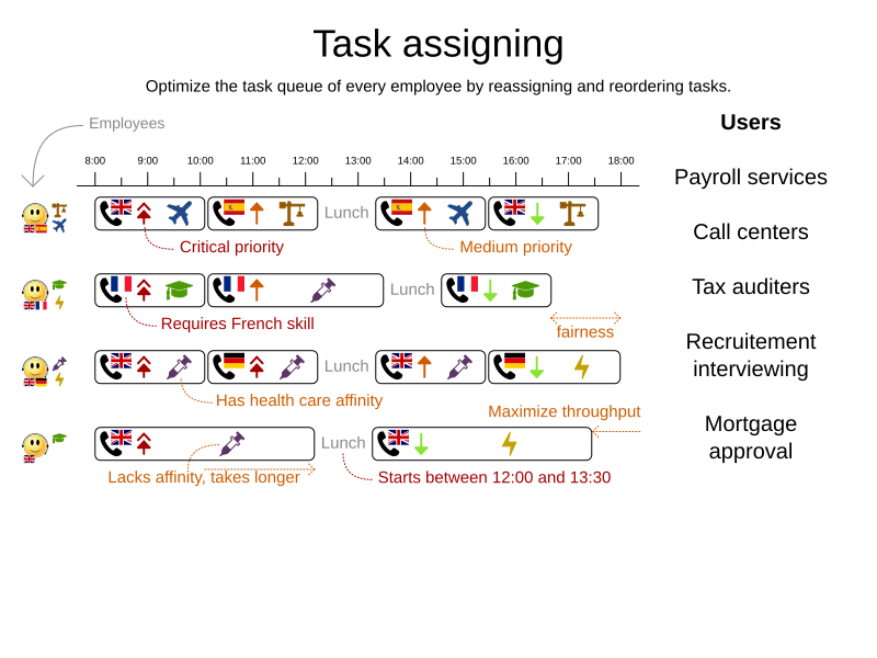
3.12.3. Problem size
24tasks-8employees   has  24 tasks, 6 skills,  8 employees,   4 task types and  4 customers with a search space of   10^30.
50tasks-5employees   has  50 tasks, 5 skills,  5 employees,  10 task types and 10 customers with a search space of   10^69.
100tasks-5employees  has 100 tasks, 5 skills,  5 employees,  20 task types and 15 customers with a search space of  10^164.
500tasks-20employees has 500 tasks, 6 skills, 20 employees, 100 task types and 60 customers with a search space of 10^1168.
3.13. Exam timetabling (ITC 2007 track 1 - Examination)
3.13.1. Problem description
Schedule each exam into a period and into a room. Multiple exams can share the same room during the same period.
Hard constraints:
-
Exam conflict: two exams that share students must not occur in the same period.
-
Room capacity: A room’s seating capacity must suffice at all times.
-
Period duration: A period’s duration must suffice for all of its exams.
-
Period related hard constraints (specified per dataset):
-
Coincidence: two specified exams must use the same period (but possibly another room).
-
Exclusion: two specified exams must not use the same period.
-
After: A specified exam must occur in a period after another specified exam’s period.
-
-
Room related hard constraints (specified per dataset):
-
Exclusive: one specified exam should not have to share its room with any other exam.
-
Soft constraints (each of which has a parametrized penalty):
-
The same student should not have two exams in a row.
-
The same student should not have two exams on the same day.
-
Period spread: two exams that share students should be a number of periods apart.
-
Mixed durations: two exams that share a room should not have different durations.
-
Front load: Large exams should be scheduled earlier in the schedule.
-
Period penalty (specified per dataset): Some periods have a penalty when used.
-
Room penalty (specified per dataset): Some rooms have a penalty when used.
It uses large test data sets of real-life universities.
The problem is defined by the International Timetabling Competition 2007 track 1. Geoffrey De Smet finished 4th in that competition with a very early version of OptaPlanner. Many improvements have been made since then.
3.13.2. Problem size
exam_comp_set1 has  7883 students,  607 exams, 54 periods,  7 rooms,  12 period constraints and  0 room constraints with a search space of 10^1564.
exam_comp_set2 has 12484 students,  870 exams, 40 periods, 49 rooms,  12 period constraints and  2 room constraints with a search space of 10^2864.
exam_comp_set3 has 16365 students,  934 exams, 36 periods, 48 rooms, 168 period constraints and 15 room constraints with a search space of 10^3023.
exam_comp_set4 has  4421 students,  273 exams, 21 periods,  1 rooms,  40 period constraints and  0 room constraints with a search space of  10^360.
exam_comp_set5 has  8719 students, 1018 exams, 42 periods,  3 rooms,  27 period constraints and  0 room constraints with a search space of 10^2138.
exam_comp_set6 has  7909 students,  242 exams, 16 periods,  8 rooms,  22 period constraints and  0 room constraints with a search space of  10^509.
exam_comp_set7 has 13795 students, 1096 exams, 80 periods, 15 rooms,  28 period constraints and  0 room constraints with a search space of 10^3374.
exam_comp_set8 has  7718 students,  598 exams, 80 periods,  8 rooms,  20 period constraints and  1 room constraints with a search space of 10^1678.
3.13.3. Domain model
Below you can see the main examination domain classes:
Notice that we’ve split up the exam concept into an Exam class and a Topic class.
The Exam instances change during solving (this is the planning entity class), when their period or room property changes.
The Topic, Period and Room instances never change during solving (these are problem facts, just like some other classes).
3.14. Nurse rostering (INRC 2010)
3.14.1. Problem description
For each shift, assign a nurse to work that shift.
Hard constraints:
-
No unassigned shifts (built-in): Every shift need to be assigned to an employee.
-
Shift conflict: An employee can have only one shift per day.
Soft constraints:
-
Contract obligations. The business frequently violates these, so they decided to define these as soft constraints instead of hard constraints.
-
Minimum and maximum assignments: Each employee needs to work more than x shifts and less than y shifts (depending on their contract).
-
Minimum and maximum consecutive working days: Each employee needs to work between x and y days in a row (depending on their contract).
-
Minimum and maximum consecutive free days: Each employee needs to be free between x and y days in a row (depending on their contract).
-
Minimum and maximum consecutive working weekends: Each employee needs to work between x and y weekends in a row (depending on their contract).
-
Complete weekends: Each employee needs to work every day in a weekend or not at all.
-
Identical shift types during weekend: Each weekend shift for the same weekend of the same employee must be the same shift type.
-
Unwanted patterns: A combination of unwanted shift types in a row. For example: a late shift followed by an early shift followed by a late shift.
-
-
Employee wishes:
-
Day on request: An employee wants to work on a specific day.
-
Day off request: An employee does not want to work on a specific day.
-
Shift on request: An employee wants to be assigned to a specific shift.
-
Shift off request: An employee does not want to be assigned to a specific shift.
-
-
Alternative skill: An employee assigned to a shift should have a proficiency in every skill required by that shift.
The problem is defined by the International Nurse Rostering Competition 2010.
3.14.3. Problem size
There are three dataset types:
-
sprint: must be solved in seconds.
-
medium: must be solved in minutes.
-
long: must be solved in hours.
toy1          has 1 skills, 3 shiftTypes, 2 patterns, 1 contracts,  6 employees,  7 shiftDates,  35 shiftAssignments and   0 requests with a search space of   10^27.
toy2          has 1 skills, 3 shiftTypes, 3 patterns, 2 contracts, 20 employees, 28 shiftDates, 180 shiftAssignments and 140 requests with a search space of  10^234.

sprint01      has 1 skills, 4 shiftTypes, 3 patterns, 4 contracts, 10 employees, 28 shiftDates, 152 shiftAssignments and 150 requests with a search space of  10^152.
sprint02      has 1 skills, 4 shiftTypes, 3 patterns, 4 contracts, 10 employees, 28 shiftDates, 152 shiftAssignments and 150 requests with a search space of  10^152.
sprint03      has 1 skills, 4 shiftTypes, 3 patterns, 4 contracts, 10 employees, 28 shiftDates, 152 shiftAssignments and 150 requests with a search space of  10^152.
sprint04      has 1 skills, 4 shiftTypes, 3 patterns, 4 contracts, 10 employees, 28 shiftDates, 152 shiftAssignments and 150 requests with a search space of  10^152.
sprint05      has 1 skills, 4 shiftTypes, 3 patterns, 4 contracts, 10 employees, 28 shiftDates, 152 shiftAssignments and 150 requests with a search space of  10^152.
sprint06      has 1 skills, 4 shiftTypes, 3 patterns, 4 contracts, 10 employees, 28 shiftDates, 152 shiftAssignments and 150 requests with a search space of  10^152.
sprint07      has 1 skills, 4 shiftTypes, 3 patterns, 4 contracts, 10 employees, 28 shiftDates, 152 shiftAssignments and 150 requests with a search space of  10^152.
sprint08      has 1 skills, 4 shiftTypes, 3 patterns, 4 contracts, 10 employees, 28 shiftDates, 152 shiftAssignments and 150 requests with a search space of  10^152.
sprint09      has 1 skills, 4 shiftTypes, 3 patterns, 4 contracts, 10 employees, 28 shiftDates, 152 shiftAssignments and 150 requests with a search space of  10^152.
sprint10      has 1 skills, 4 shiftTypes, 3 patterns, 4 contracts, 10 employees, 28 shiftDates, 152 shiftAssignments and 150 requests with a search space of  10^152.
sprint_hint01 has 1 skills, 4 shiftTypes, 8 patterns, 3 contracts, 10 employees, 28 shiftDates, 152 shiftAssignments and 150 requests with a search space of  10^152.
sprint_hint02 has 1 skills, 4 shiftTypes, 0 patterns, 3 contracts, 10 employees, 28 shiftDates, 152 shiftAssignments and 150 requests with a search space of  10^152.
sprint_hint03 has 1 skills, 4 shiftTypes, 8 patterns, 3 contracts, 10 employees, 28 shiftDates, 152 shiftAssignments and 150 requests with a search space of  10^152.
sprint_late01 has 1 skills, 4 shiftTypes, 8 patterns, 3 contracts, 10 employees, 28 shiftDates, 152 shiftAssignments and 150 requests with a search space of  10^152.
sprint_late02 has 1 skills, 3 shiftTypes, 4 patterns, 3 contracts, 10 employees, 28 shiftDates, 144 shiftAssignments and 139 requests with a search space of  10^144.
sprint_late03 has 1 skills, 4 shiftTypes, 8 patterns, 3 contracts, 10 employees, 28 shiftDates, 160 shiftAssignments and 150 requests with a search space of  10^160.
sprint_late04 has 1 skills, 4 shiftTypes, 8 patterns, 3 contracts, 10 employees, 28 shiftDates, 160 shiftAssignments and 150 requests with a search space of  10^160.
sprint_late05 has 1 skills, 4 shiftTypes, 8 patterns, 3 contracts, 10 employees, 28 shiftDates, 152 shiftAssignments and 150 requests with a search space of  10^152.
sprint_late06 has 1 skills, 4 shiftTypes, 0 patterns, 3 contracts, 10 employees, 28 shiftDates, 152 shiftAssignments and 150 requests with a search space of  10^152.
sprint_late07 has 1 skills, 4 shiftTypes, 0 patterns, 3 contracts, 10 employees, 28 shiftDates, 152 shiftAssignments and 150 requests with a search space of  10^152.
sprint_late08 has 1 skills, 4 shiftTypes, 0 patterns, 3 contracts, 10 employees, 28 shiftDates, 152 shiftAssignments and   0 requests with a search space of  10^152.
sprint_late09 has 1 skills, 4 shiftTypes, 0 patterns, 3 contracts, 10 employees, 28 shiftDates, 152 shiftAssignments and   0 requests with a search space of  10^152.
sprint_late10 has 1 skills, 4 shiftTypes, 0 patterns, 3 contracts, 10 employees, 28 shiftDates, 152 shiftAssignments and 150 requests with a search space of  10^152.

medium01      has 1 skills, 4 shiftTypes, 0 patterns, 4 contracts, 31 employees, 28 shiftDates, 608 shiftAssignments and 403 requests with a search space of  10^906.
medium02      has 1 skills, 4 shiftTypes, 0 patterns, 4 contracts, 31 employees, 28 shiftDates, 608 shiftAssignments and 403 requests with a search space of  10^906.
medium03      has 1 skills, 4 shiftTypes, 0 patterns, 4 contracts, 31 employees, 28 shiftDates, 608 shiftAssignments and 403 requests with a search space of  10^906.
medium04      has 1 skills, 4 shiftTypes, 0 patterns, 4 contracts, 31 employees, 28 shiftDates, 608 shiftAssignments and 403 requests with a search space of  10^906.
medium05      has 1 skills, 4 shiftTypes, 0 patterns, 4 contracts, 31 employees, 28 shiftDates, 608 shiftAssignments and 403 requests with a search space of  10^906.
medium_hint01 has 1 skills, 4 shiftTypes, 7 patterns, 4 contracts, 30 employees, 28 shiftDates, 428 shiftAssignments and 390 requests with a search space of  10^632.
medium_hint02 has 1 skills, 4 shiftTypes, 7 patterns, 3 contracts, 30 employees, 28 shiftDates, 428 shiftAssignments and 390 requests with a search space of  10^632.
medium_hint03 has 1 skills, 4 shiftTypes, 7 patterns, 4 contracts, 30 employees, 28 shiftDates, 428 shiftAssignments and 390 requests with a search space of  10^632.
medium_late01 has 1 skills, 4 shiftTypes, 7 patterns, 4 contracts, 30 employees, 28 shiftDates, 424 shiftAssignments and 390 requests with a search space of  10^626.
medium_late02 has 1 skills, 4 shiftTypes, 7 patterns, 3 contracts, 30 employees, 28 shiftDates, 428 shiftAssignments and 390 requests with a search space of  10^632.
medium_late03 has 1 skills, 4 shiftTypes, 0 patterns, 4 contracts, 30 employees, 28 shiftDates, 428 shiftAssignments and 390 requests with a search space of  10^632.
medium_late04 has 1 skills, 4 shiftTypes, 7 patterns, 3 contracts, 30 employees, 28 shiftDates, 416 shiftAssignments and 390 requests with a search space of  10^614.
medium_late05 has 2 skills, 5 shiftTypes, 7 patterns, 4 contracts, 30 employees, 28 shiftDates, 452 shiftAssignments and 390 requests with a search space of  10^667.

long01        has 2 skills, 5 shiftTypes, 3 patterns, 3 contracts, 49 employees, 28 shiftDates, 740 shiftAssignments and 735 requests with a search space of 10^1250.
long02        has 2 skills, 5 shiftTypes, 3 patterns, 3 contracts, 49 employees, 28 shiftDates, 740 shiftAssignments and 735 requests with a search space of 10^1250.
long03        has 2 skills, 5 shiftTypes, 3 patterns, 3 contracts, 49 employees, 28 shiftDates, 740 shiftAssignments and 735 requests with a search space of 10^1250.
long04        has 2 skills, 5 shiftTypes, 3 patterns, 3 contracts, 49 employees, 28 shiftDates, 740 shiftAssignments and 735 requests with a search space of 10^1250.
long05        has 2 skills, 5 shiftTypes, 3 patterns, 3 contracts, 49 employees, 28 shiftDates, 740 shiftAssignments and 735 requests with a search space of 10^1250.
long_hint01   has 2 skills, 5 shiftTypes, 9 patterns, 3 contracts, 50 employees, 28 shiftDates, 740 shiftAssignments and   0 requests with a search space of 10^1257.
long_hint02   has 2 skills, 5 shiftTypes, 7 patterns, 3 contracts, 50 employees, 28 shiftDates, 740 shiftAssignments and   0 requests with a search space of 10^1257.
long_hint03   has 2 skills, 5 shiftTypes, 7 patterns, 3 contracts, 50 employees, 28 shiftDates, 740 shiftAssignments and   0 requests with a search space of 10^1257.
long_late01   has 2 skills, 5 shiftTypes, 9 patterns, 3 contracts, 50 employees, 28 shiftDates, 752 shiftAssignments and   0 requests with a search space of 10^1277.
long_late02   has 2 skills, 5 shiftTypes, 9 patterns, 4 contracts, 50 employees, 28 shiftDates, 752 shiftAssignments and   0 requests with a search space of 10^1277.
long_late03   has 2 skills, 5 shiftTypes, 9 patterns, 3 contracts, 50 employees, 28 shiftDates, 752 shiftAssignments and   0 requests with a search space of 10^1277.
long_late04   has 2 skills, 5 shiftTypes, 9 patterns, 4 contracts, 50 employees, 28 shiftDates, 752 shiftAssignments and   0 requests with a search space of 10^1277.
long_late05   has 2 skills, 5 shiftTypes, 9 patterns, 3 contracts, 50 employees, 28 shiftDates, 740 shiftAssignments and   0 requests with a search space of 10^1257.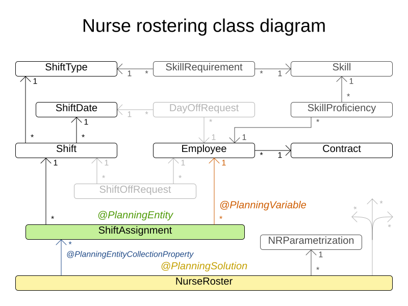
3.15. Traveling tournament problem (TTP)
3.15.1. Problem description
Schedule matches between n teams.
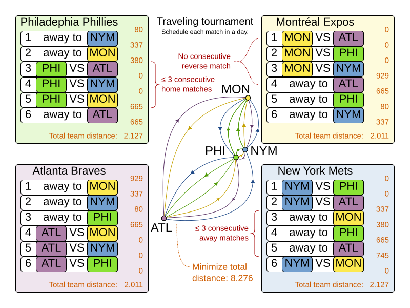
Hard constraints:
-
Each team plays twice against every other team: once home and once away.
-
Each team has exactly one match on each timeslot.
-
No team must have more than three consecutive home or three consecutive away matches.
-
No repeaters: no two consecutive matches of the same two opposing teams.
Soft constraints:
-
Minimize the total distance traveled by all teams.
The problem is defined on Michael Trick’s website (which contains the world records too).
3.15.2. Problem size
1-nl04     has  6 days,  4 teams and   12 matches with a search space of    10^5.
1-nl06     has 10 days,  6 teams and   30 matches with a search space of   10^19.
1-nl08     has 14 days,  8 teams and   56 matches with a search space of   10^43.
1-nl10     has 18 days, 10 teams and   90 matches with a search space of   10^79.
1-nl12     has 22 days, 12 teams and  132 matches with a search space of  10^126.
1-nl14     has 26 days, 14 teams and  182 matches with a search space of  10^186.
1-nl16     has 30 days, 16 teams and  240 matches with a search space of  10^259.
2-bra24    has 46 days, 24 teams and  552 matches with a search space of  10^692.
3-nfl16    has 30 days, 16 teams and  240 matches with a search space of  10^259.
3-nfl18    has 34 days, 18 teams and  306 matches with a search space of  10^346.
3-nfl20    has 38 days, 20 teams and  380 matches with a search space of  10^447.
3-nfl22    has 42 days, 22 teams and  462 matches with a search space of  10^562.
3-nfl24    has 46 days, 24 teams and  552 matches with a search space of  10^692.
3-nfl26    has 50 days, 26 teams and  650 matches with a search space of  10^838.
3-nfl28    has 54 days, 28 teams and  756 matches with a search space of  10^999.
3-nfl30    has 58 days, 30 teams and  870 matches with a search space of 10^1175.
3-nfl32    has 62 days, 32 teams and  992 matches with a search space of 10^1367.
4-super04  has  6 days,  4 teams and   12 matches with a search space of    10^5.
4-super06  has 10 days,  6 teams and   30 matches with a search space of   10^19.
4-super08  has 14 days,  8 teams and   56 matches with a search space of   10^43.
4-super10  has 18 days, 10 teams and   90 matches with a search space of   10^79.
4-super12  has 22 days, 12 teams and  132 matches with a search space of  10^126.
4-super14  has 26 days, 14 teams and  182 matches with a search space of  10^186.
5-galaxy04 has  6 days,  4 teams and   12 matches with a search space of    10^5.
5-galaxy06 has 10 days,  6 teams and   30 matches with a search space of   10^19.
5-galaxy08 has 14 days,  8 teams and   56 matches with a search space of   10^43.
5-galaxy10 has 18 days, 10 teams and   90 matches with a search space of   10^79.
5-galaxy12 has 22 days, 12 teams and  132 matches with a search space of  10^126.
5-galaxy14 has 26 days, 14 teams and  182 matches with a search space of  10^186.
5-galaxy16 has 30 days, 16 teams and  240 matches with a search space of  10^259.
5-galaxy18 has 34 days, 18 teams and  306 matches with a search space of  10^346.
5-galaxy20 has 38 days, 20 teams and  380 matches with a search space of  10^447.
5-galaxy22 has 42 days, 22 teams and  462 matches with a search space of  10^562.
5-galaxy24 has 46 days, 24 teams and  552 matches with a search space of  10^692.
5-galaxy26 has 50 days, 26 teams and  650 matches with a search space of  10^838.
5-galaxy28 has 54 days, 28 teams and  756 matches with a search space of  10^999.
5-galaxy30 has 58 days, 30 teams and  870 matches with a search space of 10^1175.
5-galaxy32 has 62 days, 32 teams and  992 matches with a search space of 10^1367.
5-galaxy34 has 66 days, 34 teams and 1122 matches with a search space of 10^1576.
5-galaxy36 has 70 days, 36 teams and 1260 matches with a search space of 10^1801.
5-galaxy38 has 74 days, 38 teams and 1406 matches with a search space of 10^2042.
5-galaxy40 has 78 days, 40 teams and 1560 matches with a search space of 10^2301.
3.16. Conference scheduling
3.16.1. Problem description
Assign each conference talk to a timeslot and a room, after the talks have been accepted.
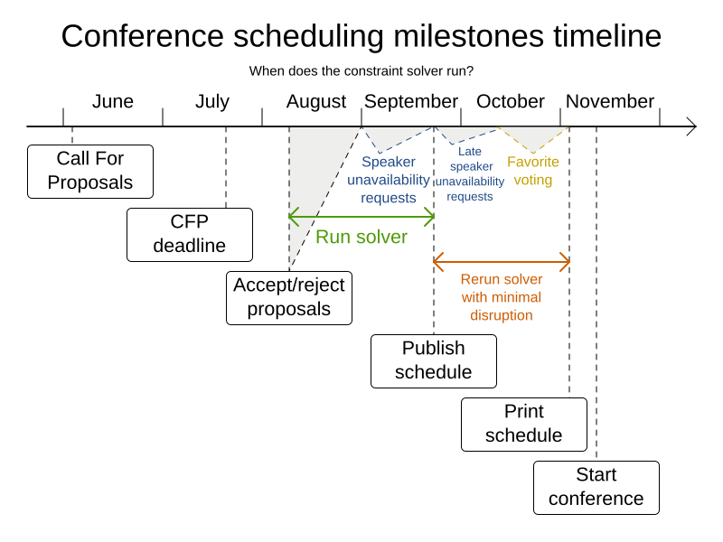
Timeslots can overlap. It reads/writes to/from an *.xlsx file that can be edited with LibreOffice or Excel.
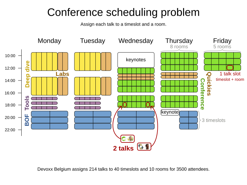
Built-in hard constraints:
-
Talk type of timeslot: The type of a talk must match the timeslot’s talk type.
-
Room unavailable timeslots: A talk’s room must be available during the talk’s timeslot.
Hard constraints (unless configured otherwise):
-
Room conflict: Two talks can’t use the same room during overlapping timeslots.
-
Speaker unavailable timeslots: Every talk’s speaker must be available during the talk’s timeslot.
-
Speaker conflict: Two talks can’t share a speaker during overlapping timeslots.
-
Talk prerequisite talks: A talk must be scheduled after all its prerequisite talks.
-
Talk mutually-exclusive-talks tags: Talks that share such tags must not be scheduled in overlapping timeslots.
-
Consecutive talks pause: A speaker who has more than one talk must have a break between them.
-
Generic purpose timeslot and room tags
-
Speaker required timeslot tags: If a speaker has a required timeslot tag, then all his/her talks must be assigned to a timeslot with that tag.
-
Speaker prohibited timeslot tags: If a speaker has a prohibited timeslot tag, then all his/her talks cannot be assigned to a timeslot with that tag.
-
Talk required timeslot tags: If a talk has a required timeslot tag, then it must be assigned to a timeslot with that tag.
-
Talk prohibited timeslot tags: If a talk has a prohibited timeslot tag, then it cannot be assigned to a timeslot with that tag.
-
Speaker required room tags: If a speaker has a required room tag, then all his/her talks must be assigned to a room with that tag.
-
Speaker prohibited room tags: If a speaker has a prohibited room tag, then all his/her talks cannot be assigned to a room with that tag.
-
Talk required room tags: If a talk has a required room tag, then it must be assigned to a room with that tag.
-
Talk prohibited room tags: If a talk has a prohibited room tag, then it cannot be assigned to a room with that tag.
-
Medium constraints (unless configured otherwise):
-
Published timeslot: A published talk must not be scheduled at a different timeslot than currently published. If a hard constraint’s input data changes after publishing (such as speaker unavailability), then this medium constraint will be minimally broken to attain a new feasible solution.
Soft constraints (unless configured otherwise):
-
Published room: Minimize the number of talks scheduled in different rooms than published ones.
-
Theme track conflict: Minimize the number of talks that share a same theme tag during overlapping timeslots.
-
Theme track room stability: Talks with common theme track tag should be scheduled in the same room throughout the day.
-
Sector conflict: Minimize the number of talks that share a same sector tag during overlapping timeslots.
-
Content audience level flow violation: For every content tag, schedule the introductory talks before the advanced talks.
-
Audience level diversity: For every timeslot, maximize the number of talks with a different audience level.
-
Language diversity: For every timeslot, maximize the number of talks with a different language.
-
Same day talks: All talks that share a theme track tag or content tag should be scheduled in the minimum number of days (ideally in the same day).
-
Popular talks: Talks with higher
favoriteCountshould be scheduled in larger rooms. -
Crowd control: Talks with higher
crowdControlRiskshould be scheduled in pairs at the same timeslot to avoid having most participants going to the same room. -
Generic purpose timeslot and room tags
-
Speaker preferred timeslot tag: If a speaker has a preferred timeslot tag, then all his/her talks should be assigned to a timeslot with that tag.
-
Speaker undesired timeslot tag: If a speaker has an undesired timeslot tag, then all his/her talks should not be assigned to a timeslot with that tag.
-
Talk preferred timeslot tag: If a talk has a preferred timeslot tag, then it should be assigned to a timeslot with that tag.
-
Talk undesired timeslot tag: If a talk has an undesired timeslot tag, then it should not be assigned to a timeslot with that tag.
-
Speaker preferred room tag: If a speaker has a preferred room tag, then all his/her talks should be assigned to a room with that tag.
-
Speaker undesired room tag: If a speaker has an undesired room tag, then all his/her talks should not be assigned to a room with that tag.
-
Talk preferred room tag: If a talk has a preferred room tag, then it should be assigned to a room with that tag.
-
Talk undesired room tag: If a talk has an undesired room tag, then it should not be assigned to a room with that tag.
-
Every constraint can be configured to use a different score level (hard/medium/soft) or a different score weight.
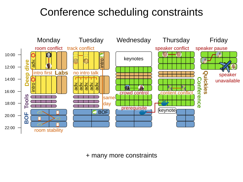
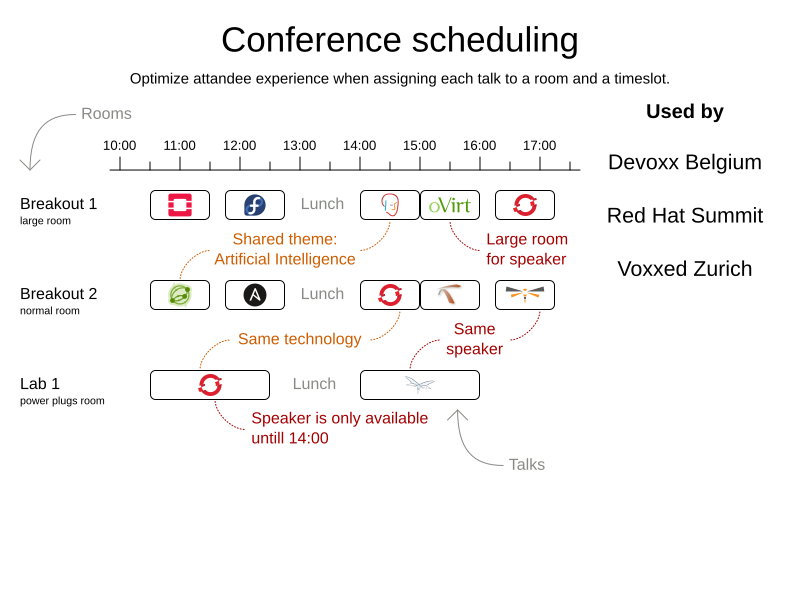
3.16.3. Problem size
18talks-6timeslots-5rooms    has  18 talks,  6 timeslots and  5 rooms with a search space of  10^26.
36talks-12timeslots-5rooms   has  36 talks, 12 timeslots and  5 rooms with a search space of  10^64.
72talks-12timeslots-10rooms  has  72 talks, 12 timeslots and 10 rooms with a search space of 10^149.
108talks-18timeslots-10rooms has 108 talks, 18 timeslots and 10 rooms with a search space of 10^243.
216talks-18timeslots-20rooms has 216 talks, 18 timeslots and 20 rooms with a search space of 10^552.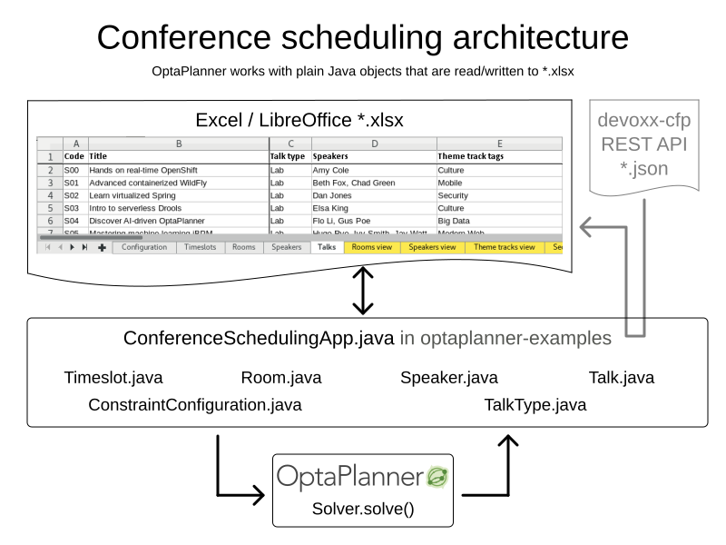
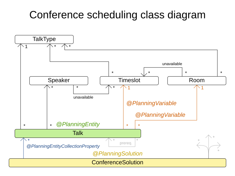
3.17. Flight crew scheduling
3.17.1. Problem description
Assign flights to pilots and flight attendants.
Hard constraints:
-
Required skill: each flight assignment has a required skill. For example, flight AB0001 requires 2 pilots and 3 flight attendants.
-
Flight conflict: each employee can only attend one flight at the same time
-
Transfer between two flights: between two flights, an employee must be able to transfer from the arrival airport to the departure airport. For example, Ann arrives in Brussels at 10:00 and departs in Amsterdam at 15:00.
-
Employee unavailability: the employee must be available on the day of the flight. For example, Ann is on vacation on 1-Feb.
Soft constraints:
-
First assignment departing from home
-
Last assignment arriving at home
-
Load balance flight duration total per employee
3.17.2. Problem size
175flights-7days-Europe  has 2 skills, 50 airports, 150 employees, 175 flights and  875 flight assignments with a search space of  10^1904.
700flights-28days-Europe has 2 skills, 50 airports, 150 employees, 700 flights and 3500 flight assignments with a search space of  10^7616.
875flights-7days-Europe  has 2 skills, 50 airports, 750 employees, 875 flights and 4375 flight assignments with a search space of 10^12578.
175flights-7days-US      has 2 skills, 48 airports, 150 employees, 175 flights and  875 flight assignments with a search space of  10^1904.
4. OptaPlanner configuration
4.1. Overview
Solving a planning problem with OptaPlanner consists of the following steps:
-
Model your planning problem as a class annotated with the
@PlanningSolutionannotation, for example theNQueensclass. -
Configure a
Solver, for example a First Fit and Tabu Search solver for anyNQueensinstance. -
Load a problem data set from your data layer, for example a Four Queens instance. That is the planning problem.
-
Solve it with
Solver.solve(problem)which returns the best solution found.
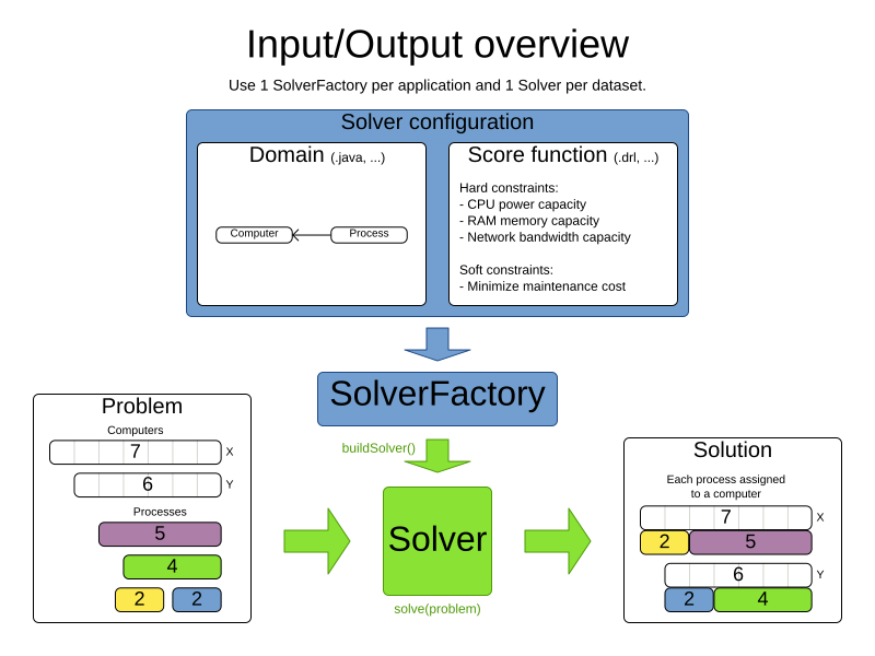
4.2. Solver configuration
4.2.1. Solver configuration by XML
Build a Solver instance with the SolverFactory.
Configure the SolverFactory with a solver configuration XML file, provided as a classpath resource (as defined by ClassLoader.getResource()):
       SolverFactory<NQueens> solverFactory = SolverFactory.createFromXmlResource(
               "org/optaplanner/examples/nqueens/solver/nqueensSolverConfig.xml");
       Solver<NQueens> solver = solverFactory.buildSolver();
In a typical project (following the Maven directory structure),
that solverConfig XML file would be located at $PROJECT_DIR/src/main/resources/org/optaplanner/examples/nqueens/solver/nqueensSolverConfig.xml.
Alternatively, a SolverFactory can be created from a File with SolverFactory.createFromXmlFile().
However, for portability reasons, a classpath resource is recommended.
Both a Solver and a SolverFactory have a generic type called Solution_, which is the class representing a planning problem and solution.
A solver configuration XML file looks like this:
<?xml version="1.0" encoding="UTF-8"?>
<solver xmlns="https://www.optaplanner.org/xsd/solver" xmlns:xsi="http://www.w3.org/2001/XMLSchema-instance"
    xsi:schemaLocation="https://www.optaplanner.org/xsd/solver https://www.optaplanner.org/xsd/solver/solver.xsd">
  <!-- Define the model -->
  <solutionClass>org.optaplanner.examples.nqueens.domain.NQueens</solutionClass>
  <entityClass>org.optaplanner.examples.nqueens.domain.Queen</entityClass>

  <!-- Define the score function -->
  <scoreDirectorFactory>
    <constraintProviderClass>org.optaplanner.examples.nqueens.score.NQueensConstraintProvider</constraintProviderClass>
  </scoreDirectorFactory>

  <!-- Configure the optimization algorithms (optional) -->
  <termination>
    ...
  </termination>
  <constructionHeuristic>
    ...
  </constructionHeuristic>
  <localSearch>
    ...
  </localSearch>
</solver>
Notice the three parts in it:
-
Define the model.
-
Define the score function.
-
Optionally configure the optimization algorithm(s).
These various parts of a configuration are explained further in this manual.
OptaPlanner makes it relatively easy to switch optimization algorithm(s) just by changing the configuration. There is even a Benchmarker which allows you to play out different configurations against each other and report the most appropriate configuration for your use case.
4.2.2. Solver configuration by Java API
A solver configuration can also be configured with the SolverConfig API.
This is especially useful to change some values dynamically at runtime.
For example, to change the running time based on system property, before building the Solver:
        SolverConfig solverConfig = SolverConfig.createFromXmlResource(
                "org/optaplanner/examples/nqueens/solver/nqueensSolverConfig.xml");
        solverConfig.withTerminationConfig(new TerminationConfig()
                        .withMinutesSpentLimit(userInput));

        SolverFactory<NQueens> solverFactory = SolverFactory.create(solverConfig);
        Solver<NQueens> solver = solverFactory.buildSolver();
Every element in the solver configuration XML is available as a *Config class
or a property on a *Config class in the package namespace org.optaplanner.core.config.
These *Config classes are the Java representation of the XML format.
They build the runtime components (of the package namespace org.optaplanner.core.impl)
and assemble them into an efficient Solver.
|
To configure a |
4.2.3. Annotation alternatives
OptaPlanner needs to be told which classes in your domain model are planning entities, which properties are planning variables, etc. There are several ways to deliver this information:
-
Add class annotations and JavaBean property annotations on the domain model (recommended). The property annotations must be on the getter method, not on the setter method. Such a getter does not need to be public.
-
Add class annotations and field annotations on the domain model. Such a field does not need to be public.
-
No annotations: externalize the domain configuration in an XML file. This is not yet supported.
This manual focuses on the first manner, but every feature supports all three manners, even if it’s not explicitly mentioned.
4.2.4. Domain access
OptaPlanner by default accesses your domain using reflection, which will always work, but is slow compared to direct access. Alternatively, you can configure OptaPlanner to access your domain using Gizmo, which will generate bytecode that directly access the fields/methods of your domain without reflection. However, it comes with some restrictions:
-
All fields in the domain must be public.
-
The planning annotations can only be on public fields and public getters.
-
io.quarkus.gizmo:gizmo must be on the classpath.
These restrictions do not apply when using OptaPlanner with Quarkus, where Gizmo is the default domain access type.
To use Gizmo outside of Quarkus, set the domainAccessType in the
Solver Configuration:
  <solver>
    <domainAccessType>GIZMO</domainAccessType>
  </solver>
4.2.5. Custom properties configuration
Solver configuration elements, that instantiate classes and explicitly mention it, support custom properties.
Custom properties are useful to tweak dynamic values through the Benchmarker.
For example, presume your EasyScoreCalculator has heavy calculations (which are cached)
and you want to increase the cache size in one benchmark:
  <scoreDirectorFactory>
    <easyScoreCalculatorClass>...MyEasyScoreCalculator</easyScoreCalculatorClass>
    <easyScoreCalculatorCustomProperties>
      <property name="myCacheSize" value="1000"/><!-- Override value -->
    </easyScoreCalculatorCustomProperties>
  </scoreDirectorFactory>
Add a public setter for each custom property, which is called when a Solver is built.
public class MyEasyScoreCalculator extends EasyScoreCalculator<MySolution, SimpleScore> {

        private int myCacheSize = 500; // Default value

        @SuppressWarnings("unused")
        public void setMyCacheSize(int myCacheSize) {
            this.myCacheSize = myCacheSize;
        }

    ...
}
Most value types are supported (including boolean, int, double, BigDecimal, String and enums).
4.3. Model a planning problem
4.3.1. Is this class a problem fact or planning entity?
Look at a dataset of your planning problem. You will recognize domain classes in there, each of which can be categorized as one of the following:
-
An unrelated class: not used by any of the score constraints. From a planning standpoint, this data is obsolete.
-
A problem fact class: used by the score constraints, but does NOT change during planning (as long as the problem stays the same). For example:
Bed,Room,Shift,Employee,Topic,Period, … All the properties of a problem fact class are problem properties. -
A planning entity class: used by the score constraints and changes during planning. For example:
BedDesignation,ShiftAssignment,Exam, … The properties that change during planning are planning variables. The other properties are problem properties.
Ask yourself: What class changes during planning? Which class has variables that I want the Solver to change for me? That class is a planning entity.
Most use cases have only one planning entity class.
Most use cases also have only one planning variable per planning entity class.
|
In real-time planning, even though the problem itself changes, problem facts do not really change during planning, instead they change between planning (because the Solver temporarily stops to apply the problem fact changes). |
To create a good domain model, read the domain modeling guide.
In OptaPlanner, all problem facts and planning entities are plain old JavaBeans (POJOs). Load them from a database, an XML file, a data repository, a REST service, a noSQL cloud, … (see integration): it doesn’t matter.
4.3.2. Problem fact
A problem fact is any JavaBean (POJO) with getters that does not change during planning. For example in n queens, the columns and rows are problem facts:
public class Column {

    private int index;

    // ... getters
}
public class Row {
private int index;
// ... getters
}A problem fact can reference other problem facts of course:
public class Course {

    private String code;

    private Teacher teacher; // Other problem fact
    private int lectureSize;
    private int minWorkingDaySize;

    private List<Curriculum> curriculumList; // Other problem facts
    private int studentSize;

    // ... getters
}
A problem fact class does not require any OptaPlanner specific code. For example, you can reuse your domain classes, which might have JPA annotations.
|
Generally, better designed domain classes lead to simpler and more efficient score constraints.
Therefore, when dealing with a messy (denormalized) legacy system, it can sometimes be worthwhile to convert the messy domain model into a OptaPlanner specific model first.
For example: if your domain model has two Alternatively, you can sometimes also introduce a cached problem fact to enrich the domain model for planning only. |
4.3.3. Planning entity
4.3.3.1. Planning entity annotation
A planning entity is a JavaBean (POJO) that changes during solving, for example a Queen that changes to another row.
A planning problem has multiple planning entities, for example for a single n queens problem, each Queen is a planning entity.
But there is usually only one planning entity class, for example the Queen class.
A planning entity class needs to be annotated with the @PlanningEntity annotation.
Each planning entity class has one or more planning variables (which can be genuine or shadows).
It should also have one or more defining properties.
For example in n queens, a Queen is defined by its Column and has a planning variable Row.
This means that a Queen’s column never changes during solving, while its row does change.
@PlanningEntity
public class Queen {

    private Column column;

    // Planning variables: changes during planning, between score calculations.
    private Row row;

    // ... getters and setters
}
A planning entity class can have multiple planning variables.
For example, a Lecture is defined by its Course and its index in that course (because one course has multiple lectures).
Each Lecture needs to be scheduled into a Period and a Room so it has two planning variables (period and room).
For example: the course Mathematics has eight lectures per week, of which the first lecture is Monday morning at 08:00 in room 212.
@PlanningEntity
public class Lecture {

    private Course course;
    private int lectureIndexInCourse;

    // Planning variables: changes during planning, between score calculations.
    private Period period;
    private Room room;

    // ...
}
The solver configuration needs to declare each planning entity class:
<solver xmlns="https://www.optaplanner.org/xsd/solver" xmlns:xsi="http://www.w3.org/2001/XMLSchema-instance"
    xsi:schemaLocation="https://www.optaplanner.org/xsd/solver https://www.optaplanner.org/xsd/solver/solver.xsd">
  ...
  <entityClass>org.optaplanner.examples.nqueens.domain.Queen</entityClass>
  ...
</solver>
Some uses cases have multiple planning entity classes. For example: route freight and trains into railway network arcs, where each freight can use multiple trains over its journey and each train can carry multiple freights per arc. Having multiple planning entity classes directly raises the implementation complexity of your use case.
|
Do not create unnecessary planning entity classes. This leads to difficult For example, do not create a planning entity class to hold the total free time of a teacher, which needs to be kept up to date as the If historic data needs to be considered too, then create problem fact to hold the total of the historic assignments up to, but not including, the planning window (so that it does not change when a planning entity changes) and let the score constraints take it into account. |
|
Planning entity |
4.3.3.2. Planning entity difficulty
Some optimization algorithms work more efficiently if they have an estimation of which planning entities are more difficult to plan. For example: in bin packing bigger items are harder to fit, in course scheduling lectures with more students are more difficult to schedule, and in n queens the middle queens are more difficult to fit on the board.
|
Do not try to use planning entity difficulty to implement a business constraint. It will not affect the score function: if we have infinite solving time, the returned solution will be the same. To attain a schedule in which certain entities are scheduled earlier in the schedule, add a score constraint to change the score function so it prefers such solutions. Only consider adding planning entity difficulty too if it can make the solver more efficient. |
To allow the heuristics to take advantage of that domain specific information, set a difficultyComparatorClass to the @PlanningEntity annotation:
@PlanningEntity(difficultyComparatorClass = CloudProcessDifficultyComparator.class)
public class CloudProcess {
    // ...
}
public class CloudProcessDifficultyComparator implements Comparator<CloudProcess> {
public int compare(CloudProcess a, CloudProcess b) {
return new CompareToBuilder()
.append(a.getRequiredMultiplicand(), b.getRequiredMultiplicand())
.append(a.getId(), b.getId())
.toComparison();
}
}Alternatively, you can also set a difficultyWeightFactoryClass to the @PlanningEntity annotation,
so that you have access to the rest of the problem facts from the solution too:
@PlanningEntity(difficultyWeightFactoryClass = QueenDifficultyWeightFactory.class)
public class Queen {
// ...
}See sorted selection for more information.
|
Difficulty should be implemented ascending: easy entities are lower, difficult entities are higher. For example, in bin packing: small item < medium item < big item. Although most algorithms start with the more difficult entities first, they just reverse the ordering. |
None of the current planning variable states should be used to compare planning entity difficulty. During Construction Heuristics, those variables are likely to be null anyway.
For example, a Queen's row variable should not be used.
4.3.4. Planning variable (genuine)
4.3.4.1. Planning variable annotation
A planning variable is a JavaBean property (so a getter and setter) on a planning entity.
It points to a planning value, which changes during planning.
For example, a Queen's row property is a genuine planning variable.
Note that even though a Queen's row property changes to another Row during planning, no Row instance itself is changed.
Normally planning variables are genuine, but advanced cases can also have shadows.
A genuine planning variable getter needs to be annotated with the @PlanningVariable annotation, optionally with a non-empty valueRangeProviderRefs property.
@PlanningEntity
public class Queen {
...
private Row row;
@PlanningVariable
public Row getRow() {
return row;
}
public void setRow(Row row) {
this.row = row;
}
}The optional valueRangeProviderRefs property defines what are the possible planning values for this planning variable.
It references one or more @ValueRangeProvider id's.
If none are provided, OptaPlanner will attempt to auto-detect matching @ValueRangeProviders.
|
A @PlanningVariable annotation needs to be on a member in a class with a @PlanningEntity annotation. It is ignored on parent classes or subclasses without that annotation. |
Annotating the field instead of the property works too:
@PlanningEntity
public class Queen {
...
@PlanningVariable
private Row row;
}|
For more advanced planning variables used to model precedence relationships, see planning list variable and chained planning variable. |
4.3.4.2. Nullable planning variable
By default, an initialized planning variable cannot be null, so an initialized solution will never use null for any of its planning variables.
In an over-constrained use case, this can be counterproductive.
For example: in task assignment with too many tasks for the workforce, we would rather leave low priority tasks unassigned instead of assigning them to an overloaded worker.
To allow an initialized planning variable to be null, set nullable to true:
@PlanningVariable(..., nullable = true)
public Worker getWorker() {
return worker;
}|
Constraint Streams filter out planning entities with a |
OptaPlanner will automatically add the value null to the value range.
There is no need to add null in a collection provided by a ValueRangeProvider.
|
Using a nullable planning variable implies that your score calculation is responsible for punishing (or even rewarding) variables with a |
|
Currently chained planning variables are not compatible with |
Repeated planning (especially real-time planning) does not mix well with a nullable planning variable.
Every time the Solver starts or a problem fact change is made, the Construction Heuristics
will try to initialize all the null variables again, which can be a huge waste of time.
One way to deal with this is to filter the entity selector of the placer in the construction heuristic.
<solver xmlns="https://www.optaplanner.org/xsd/solver" xmlns:xsi="http://www.w3.org/2001/XMLSchema-instance"
xsi:schemaLocation="https://www.optaplanner.org/xsd/solver https://www.optaplanner.org/xsd/solver/solver.xsd">
...
<constructionHeuristic>
<queuedEntityPlacer>
<entitySelector id="entitySelector1">
<filterClass>...</filterClass>
</entitySelector>
</queuedEntityPlacer>
...
<changeMoveSelector>
<entitySelector mimicSelectorRef="entitySelector1" />
</changeMoveSelector>
...
</constructionHeuristic>
...
</solver>4.3.4.3. When is a planning variable considered initialized?
A planning variable is considered initialized if its value is not null or if the variable is nullable.
So a nullable variable is always considered initialized.
A planning entity is initialized if all of its planning variables are initialized.
A solution is initialized if all of its planning entities are initialized.
4.3.5. Planning value and planning value range
4.3.5.1. Planning value
A planning value is a possible value for a genuine planning variable.
Usually, a planning value is a problem fact, but it can also be any object, for example a double.
It can even be another planning entity or even an interface implemented by both a planning entity and a problem fact.
A planning value range is the set of possible planning values for a planning variable.
This set can be a countable (for example row 1, 2, 3 or 4) or uncountable (for example any double between 0.0 and 1.0).
4.3.5.2. Planning value range provider
4.3.5.2.1. Overview
The value range of a planning variable is defined with the @ValueRangeProvider annotation.
A @ValueRangeProvider may carry a property id, which is referenced by the @PlanningVariable's property valueRangeProviderRefs.
This annotation can be located on two types of methods:
-
On the Solution: All planning entities share the same value range.
-
On the planning entity: The value range differs per planning entity. This is less common.
|
A @ValueRangeProvider annotation needs to be on a member in a class with a @PlanningSolution or a @PlanningEntity annotation. It is ignored on parent classes or subclasses without those annotations. |
The return type of that method can be three types:
-
Collection: The value range is defined by aCollection(usually aList) of its possible values. -
Array: The value range is defined by an array of its possible values.
-
ValueRange: The value range is defined by its bounds. This is less common.
4.3.5.2.2. ValueRangeProvider on the solution
All instances of the same planning entity class share the same set of possible planning values for that planning variable. This is the most common way to configure a value range.
The @PlanningSolution implementation has method that returns a Collection (or a ValueRange).
Any value from that Collection is a possible planning value for this planning variable.
@PlanningVariable
public Row getRow() {
return row;
}@PlanningSolution
public class NQueens {
...
@ValueRangeProvider
public List<Row> getRowList() {
return rowList;
}
}|
That |
Annotating the field instead of the property works too:
@PlanningSolution
public class NQueens {
...
@ValueRangeProvider
private List<Row> rowList;
}4.3.5.2.3. ValueRangeProvider on the Planning Entity
Each planning entity has its own value range (a set of possible planning values) for the planning variable. For example, if a teacher can never teach in a room that does not belong to his department, lectures of that teacher can limit their room value range to the rooms of his department.
@PlanningVariable
public Room getRoom() {
return room;
}
@ValueRangeProvider
public List<Room> getPossibleRoomList() {
return getCourse().getTeacher().getDepartment().getRoomList();
}Never use this to enforce a soft constraint (or even a hard constraint when the problem might not have a feasible solution). For example: Unless there is no other way, a teacher cannot teach in a room that does not belong to his department. In this case, the teacher should not be limited in his room value range (because sometimes there is no other way).
|
By limiting the value range specifically of one planning entity, you are effectively creating a built-in hard constraint. This can have the benefit of severely lowering the number of possible solutions; however, it can also take away the freedom of the optimization algorithms to temporarily break that constraint in order to escape from a local optimum. |
A planning entity should not use other planning entities to determine its value range. That would only try to make the planning entity solve the planning problem itself and interfere with the optimization algorithms.
Every entity has its own List instance, unless multiple entities have the same value range.
For example, if teacher A and B belong to the same department, they use the same List<Room> instance.
Furthermore, each List contains a subset of the same set of planning value instances.
For example, if department A and B can both use room X, then their List<Room> instances contain the same Room instance.
|
A |
|
A |
|
A |
4.3.5.2.4. Referencing ValueRangeProviders
There are two ways how to match a planning variable to a value range provider. The simplest way is to have value range provider auto-detected. Another way is to explicitly reference the value range provider.
ValueRangeProvidersWe already described the first approach.
By not providing any valueRangeProviderRefs on the @PlanningVariable annotation,
OptaPlanner will go over every @ValueRangeProvider-annotated method or field which does not have an id property set,
and will match planning variables with value ranges where their types match.
In the following example,
the planning variable car will be matched to the value range returned by getCompanyCarList(),
as they both use the Car type.
It will not match getPersonalCarList(),
because that value range provider is not anonymous; it specifies an id.
@PlanningVariable
public Car getCar() {
return car;
}
@ValueRangeProvider
public List<Car> getCompanyCarList() {
return companyCarList;
}
@ValueRangeProvider(id = "personalCarRange")
public List<Car> getPersonalCarList() {
return personalCarList;
}Automatic matching also accounts for polymorphism.
In the following example,
the planning variable car will be matched to getCompanyCarList() and getPersonalCarList(),
as both CompanyCar and PersonalCar are Cars.
It will not match getAirplanes(),
as an Airplane is not a Car.
@PlanningVariable
public Car getCar() {
return car;
}
@ValueRangeProvider
public List<CompanyCar> getCompanyCarList() {
return companyCarList;
}
@ValueRangeProvider
public List<PersonalCar> getPersonalCarList() {
return personalCarList;
}
@ValueRangeProvider
public List<Airplane> getAirplanes() {
return airplaneList;
}ValueRangeProvidersIn more complicated cases where auto-detection is not sufficient or where clarity is preferred over simplicity, value range providers can also be referenced explicitly.
In the following example,
the car planning variable will only be matched to value range provided by methods getCompanyCarList().
@PlanningVariable(valueRangeProviderRefs = {"companyCarRange"})
public Car getCar() {
return car;
}
@ValueRangeProvider(id = "companyCarRange")
public List<CompanyCar> getCompanyCarList() {
return companyCarList;
}
@ValueRangeProvider(id = "personalCarRange")
public List<PersonalCar> getPersonalCarList() {
return personalCarList;
}Explicitly referenced value range providers can also be combined, for example:
@PlanningVariable(valueRangeProviderRefs = { "companyCarRange", "personalCarRange" })
public Car getCar() {
return car;
}
@ValueRangeProvider(id = "companyCarRange")
public List<CompanyCar> getCompanyCarList() {
return companyCarList;
}
@ValueRangeProvider(id = "personalCarRange")
public List<PersonalCar> getPersonalCarList() {
return personalCarList;
}4.3.5.2.5. ValueRangeFactory
Instead of a Collection, you can also return a ValueRange or CountableValueRange, built by the ValueRangeFactory:
@ValueRangeProvider
public CountableValueRange<Integer> getDelayRange() {
return ValueRangeFactory.createIntValueRange(0, 5000);
}A ValueRange uses far less memory, because it only holds the bounds.
In the example above, a Collection would need to hold all 5000 ints, instead of just the two bounds.
Furthermore, an incrementUnit can be specified, for example if you have to buy stocks in units of 200 pieces:
@ValueRangeProvider
public CountableValueRange<Integer> getStockAmountRange() {
// Range: 0, 200, 400, 600, ..., 9999600, 9999800, 10000000
return ValueRangeFactory.createIntValueRange(0, 10000000, 200);
}|
Return |
The ValueRangeFactory has creation methods for several value class types:
-
boolean: A boolean range. -
int: A 32bit integer range. -
long: A 64bit integer range. -
double: A 64bit floating point range which only supports random selection (because it does not implementCountableValueRange). -
BigInteger: An arbitrary-precision integer range. -
BigDecimal: A decimal point range. By default, the increment unit is the lowest non-zero value in the scale of the bounds. -
Temporal(such asLocalDate,LocalDateTime, …): A time range.
4.3.5.3. Planning value strength
Some optimization algorithms work a bit more efficiently if they have an estimation of which planning values are stronger, which means they are more likely to satisfy a planning entity. For example: in bin packing bigger containers are more likely to fit an item and in course scheduling bigger rooms are less likely to break the student capacity constraint. Usually, the efficiency gain of planning value strength is far less than that of planning entity difficulty.
|
Do not try to use planning value strength to implement a business constraint. It will not affect the score function: if we have infinite solving time, the returned solution will be the same. To affect the score function, add a score constraint. Only consider adding planning value strength too if it can make the solver more efficient. |
To allow the heuristics to take advantage of that domain specific information, set a strengthComparatorClass to the @PlanningVariable annotation:
@PlanningVariable(..., strengthComparatorClass = CloudComputerStrengthComparator.class)
public CloudComputer getComputer() {
return computer;
}public class CloudComputerStrengthComparator implements Comparator<CloudComputer> {
public int compare(CloudComputer a, CloudComputer b) {
return new CompareToBuilder()
.append(a.getMultiplicand(), b.getMultiplicand())
.append(b.getCost(), a.getCost()) // Descending (but this is debatable)
.append(a.getId(), b.getId())
.toComparison();
}
}|
If you have multiple planning value classes in the same value range, the |
Alternatively, you can also set a strengthWeightFactoryClass to the @PlanningVariable annotation, so you have access to the rest of the problem facts from the solution too:
@PlanningVariable(..., strengthWeightFactoryClass = RowStrengthWeightFactory.class)
public Row getRow() {
return row;
}See sorted selection for more information.
|
Strength should be implemented ascending: weaker values are lower, stronger values are higher. For example in bin packing: small container < medium container < big container. |
None of the current planning variable state in any of the planning entities should be used to compare planning values. During construction heuristics, those variables are likely to be null.
For example, none of the row variables of any Queen may be used to determine the strength of a Row.
4.3.6. Planning list variable (VRP, Task assigning, …)
Use the planning list variable to model problems where the goal is to distribute a number of workload elements among limited resources in a specific order. This includes, for example, vehicle routing, traveling salesman, task assigning, and similar problems, that have previously been modeled using the chained planning variable.
The planning list variable is a successor to the chained planning variable and provides a more intuitive way to express the problem domain with Java classes.
|
As a new feature, planning list variable does not yet support all the advanced planning features that work with the chained planning variable. Use a chained planning variable instead of a planning list variable, if you need any of the following planning techniques:
|
For example, the vehicle routing problem can be modeled as follows:
This model is closer to the reality than the chained model. Each vehicle has a list of customers to go to in the order given by the list. And indeed, the object model matches the natural language description of the problem:
@PlanningEntity
class Vehicle {
int capacity;
Depot depot;
@PlanningListVariable
List<Customer> customers = new ArrayList<>();
}Planning list variable can be used if the domain meets the following criteria:
-
There is a one-to-many relationship between the planning entity and the planning value.
-
The order in which planning values are assigned to an entity’s list variable is significant.
-
Each planning value is assigned to exactly one planning entity. No planning value may appear in multiple entities.
4.3.7. Chained planning variable (TSP, VRP, …)
Chained planning variable is one way to implement the Chained Through Time pattern. This pattern is used for some use cases, such as TSP and vehicle routing. Use the chained planning variable to implement this pattern if you plan to use some of the advanced planning features, that are not yet supported by the planning list variable.
Chained planning variable allows the planning entities to point to each other and form a chain. By modeling the problem as a set of chains (instead of a set of trees/loops), the search space is heavily reduced.
A planning variable that is chained either:
-
Directly points to a problem fact (or planning entity), which is called an anchor.
-
Points to another planning entity with the same planning variable, which recursively points to an anchor.
Here are some examples of valid and invalid chains:
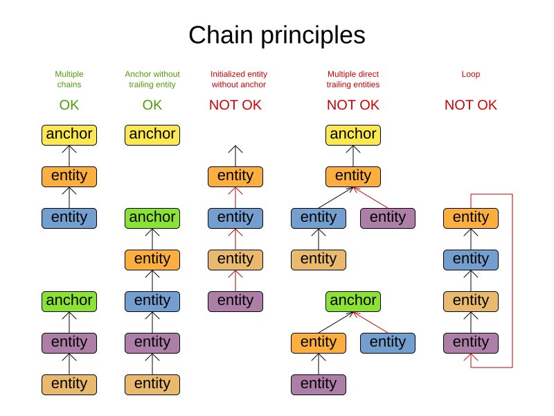
Every initialized planning entity is part of an open-ended chain that begins from an anchor. A valid model means that:
-
A chain is never a loop. The tail is always open.
-
Every chain always has exactly one anchor. The anchor is never an instance of the planning entity class that contains the chained planning variable.
-
A chain is never a tree, it is always a line. Every anchor or planning entity has at most one trailing planning entity.
-
Every initialized planning entity is part of a chain.
-
An anchor with no planning entities pointing to it, is also considered a chain.
|
A planning problem instance given to the |
|
If your constraints dictate a closed chain, model it as an open-ended chain (which is easier to persist in a database) and implement a score constraint for the last entity back to the anchor. |
The optimization algorithms and built-in Moves do chain correction to guarantee that the model stays valid:
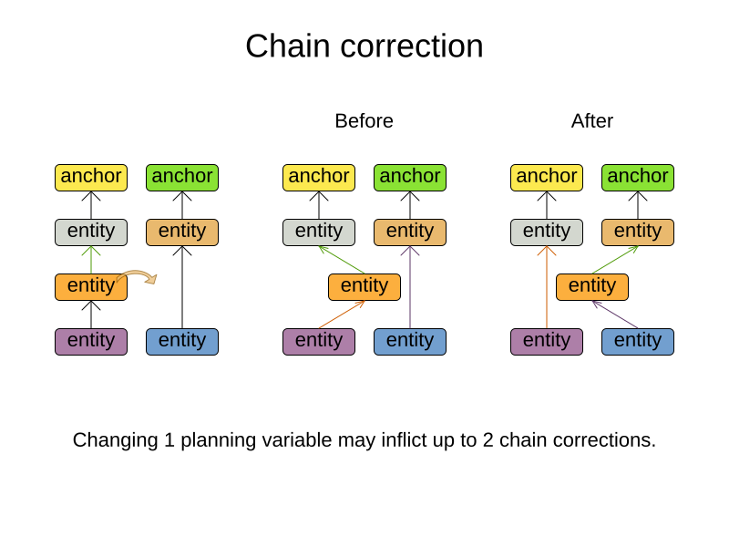
|
A custom |
For example, in TSP the anchor is a Domicile (in vehicle routing it is Vehicle):
public class Domicile ... implements Standstill {
...
public City getCity() {...}
}The anchor (which is a problem fact) and the planning entity implement a common interface, for example TSP’s Standstill:
public interface Standstill {
City getCity();
}That interface is the return type of the planning variable.
Furthermore, the planning variable is chained.
For example TSP’s Visit:
@PlanningEntity
public class Visit ... implements Standstill {
...
public City getCity() {...}
@PlanningVariable(graphType = PlanningVariableGraphType.CHAINED)
public Standstill getPreviousStandstill() {
return previousStandstill;
}
public void setPreviousStandstill(Standstill previousStandstill) {
this.previousStandstill = previousStandstill;
}
}Notice how two value range providers are usually combined:
-
The value range provider that holds the anchors, for example
domicileList. -
The value range provider that holds the initialized planning entities, for example
visitList.
4.3.8. Planning problem and planning solution
4.3.8.1. Planning problem instance
A dataset for a planning problem needs to be wrapped in a class for the Solver to solve.
That solution class represents both the planning problem and (if solved) a solution.
It is annotated with a @PlanningSolution annotation.
For example in n queens, the solution class is the NQueens class, which contains a Column list, a Row list, and a Queen list.
A planning problem is actually an unsolved planning solution or - stated differently - an uninitialized solution.
For example in n queens, that NQueens class has the @PlanningSolution annotation, yet every Queen in an unsolved NQueens class is not yet assigned to a Row (their row property is null). That’s not a feasible solution.
It’s not even a possible solution.
It’s an uninitialized solution.
4.3.8.2. Solution class
A solution class holds all problem facts, planning entities and a score.
It is annotated with a @PlanningSolution annotation.
For example, an NQueens instance holds a list of all columns, all rows and all Queen instances:
@PlanningSolution
public class NQueens {
// Problem facts
private int n;
private List<Column> columnList;
private List<Row> rowList;
// Planning entities
private List<Queen> queenList;
private SimpleScore score;
...
}The solver configuration needs to declare the planning solution class:
<solver xmlns="https://www.optaplanner.org/xsd/solver" xmlns:xsi="http://www.w3.org/2001/XMLSchema-instance"
xsi:schemaLocation="https://www.optaplanner.org/xsd/solver https://www.optaplanner.org/xsd/solver/solver.xsd">
...
<solutionClass>org.optaplanner.examples.nqueens.domain.NQueens</solutionClass>
...
</solver>4.3.8.3. Planning entities of a solution (@PlanningEntityCollectionProperty)
OptaPlanner needs to extract the entity instances from the solution instance.
It gets those collection(s) by calling every getter (or field) that is annotated with @PlanningEntityCollectionProperty:
@PlanningSolution
public class NQueens {
...
private List<Queen> queenList;
@PlanningEntityCollectionProperty
public List<Queen> getQueenList() {
return queenList;
}
}There can be multiple @PlanningEntityCollectionProperty annotated members.
Those can even return a Collection with the same entity class type.
Instead of Collection, it can also return an array.
|
A |
In rare cases, a planning entity might be a singleton: use @PlanningEntityProperty on its getter (or field) instead.
Both annotations can also be auto discovered if enabled.
4.3.8.4. Score of a Solution (@PlanningScore)
A @PlanningSolution class requires a score property (or field), which is annotated with a @PlanningScore annotation.
The score property is null if the score hasn’t been calculated yet.
The score property is typed to the specific Score implementation of your use case.
For example, NQueens uses a SimpleScore:
@PlanningSolution
public class NQueens {
...
private SimpleScore score;
@PlanningScore
public SimpleScore getScore() {
return score;
}
public void setScore(SimpleScore score) {
this.score = score;
}
}Most use cases use a HardSoftScore instead:
@PlanningSolution
public class CloudBalance {
...
private HardSoftScore score;
@PlanningScore
public HardSoftScore getScore() {
return score;
}
public void setScore(HardSoftScore score) {
this.score = score;
}
}Some use cases use other score types.
This annotation can also be auto discovered if enabled.
4.3.8.5. Problem facts of a solution (@ProblemFactCollectionProperty)
For Constraint Streams and Drools score calculation (Deprecated),
OptaPlanner needs to extract the problem fact instances from the solution instance.
It gets those collection(s) by calling every method (or field) that is annotated with @ProblemFactCollectionProperty.
All objects returned by those methods are available to use by Constraint Streams or Drools rules.
For example in NQueens all Column and Row instances are problem facts.
@PlanningSolution
public class NQueens {
...
private List<Column> columnList;
private List<Row> rowList;
@ProblemFactCollectionProperty
public List<Column> getColumnList() {
return columnList;
}
@ProblemFactCollectionProperty
public List<Row> getRowList() {
return rowList;
}
}All planning entities are automatically inserted into the working memory. Do not add an annotation on their properties.
|
The problem facts methods are not called often: at most only once per solver phase per solver thread. |
There can be multiple @ProblemFactCollectionProperty annotated members.
Those can even return a Collection with the same class type, but they shouldn’t return the same instance twice.
Instead of Collection, it can also return an array.
|
A @ProblemFactCollectionProperty annotation needs to be on a member in a class with a @PlanningSolution annotation. It is ignored on parent classes or subclasses without that annotation. |
In rare cases, a problem fact might be a singleton: use @ProblemFactProperty on its method (or field) instead.
Both annotations can also be auto discovered if enabled.
4.3.8.5.1. Cached problem fact
A cached problem fact is a problem fact that does not exist in the real domain model, but is calculated before the Solver really starts solving.
The problem facts methods have the opportunity to enrich the domain model with such cached problem facts, which can lead to simpler and faster score constraints.
For example in examination, a cached problem fact TopicConflict is created for every two Topics which share at least one Student.
@ProblemFactCollectionProperty
private List<TopicConflict> calculateTopicConflictList() {
List<TopicConflict> topicConflictList = new ArrayList<TopicConflict>();
for (Topic leftTopic : topicList) {
for (Topic rightTopic : topicList) {
if (leftTopic.getId() < rightTopic.getId()) {
int studentSize = 0;
for (Student student : leftTopic.getStudentList()) {
if (rightTopic.getStudentList().contains(student)) {
studentSize++;
}
}
if (studentSize > 0) {
topicConflictList.add(new TopicConflict(leftTopic, rightTopic, studentSize));
}
}
}
}
return topicConflictList;
}Where a score constraint needs to check that no two exams with a topic that shares a student are scheduled close together (depending on the constraint: at the same time, in a row, or in the same day), the TopicConflict instance can be used as a problem fact, rather than having to combine every two Student instances.
4.3.8.6. Auto discover solution properties
Instead of configuring each property (or field) annotation explicitly, some can also be deduced automatically by OptaPlanner. For example, on the cloud balancing example:
@PlanningSolution(autoDiscoverMemberType = AutoDiscoverMemberType.FIELD)
public class CloudBalance {
// Auto discovered as @ProblemFactCollectionProperty
@ValueRangeProvider
private List<CloudComputer> computerList;
// Auto discovered as @PlanningEntityCollectionProperty
private List<CloudProcess> processList;
// Auto discovered as @PlanningScore
private HardSoftScore score;
...
}The AutoDiscoverMemberType can be:
-
NONE: No auto discovery. -
FIELD: Auto discover all fields on the@PlanningSolutionclass -
GETTER: Auto discover all getters on the@PlanningSolutionclass
The automatic annotation is based on the field type (or getter return type):
-
@ProblemFactProperty: when it isn’t aCollection, an array, a@PlanningEntityclass or aScore -
@ProblemFactCollectionProperty: when it’s aCollection(or array) of a type that isn’t a@PlanningEntityclass -
@PlanningEntityProperty: when it is a configured@PlanningEntityclass or subclass -
@PlanningEntityCollectionProperty: when it’s aCollection(or array) of a type that is a configured@PlanningEntityclass or subclass -
@PlanningScore: when it is aScoreor subclass
These automatic annotations can still be overwritten per field (or getter).
Specifically, a BendableScore always needs to override
with an explicit @PlanningScore annotation to define the number of hard and soft levels.
4.3.8.7. Cloning a solution
Most (if not all) optimization algorithms clone the solution each time they encounter a new best solution (so they can recall it later) or to work with multiple solutions in parallel.
|
There are many ways to clone, such as a shallow clone, deep clone, … This context focuses on a planning clone. |
A planning clone of a solution must fulfill these requirements:
-
The clone must represent the same planning problem. Usually it reuses the same instances of the problem facts and problem fact collections as the original.
-
The clone must use different, cloned instances of the entities and entity collections. Changes to an original solution entity’s variables must not affect its clone.
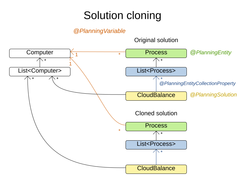
Implementing a planning clone method is hard, therefore you do not need to implement it.
4.3.8.7.1. FieldAccessingSolutionCloner
This SolutionCloner is used by default.
It works well for most use cases.
|
When the |
The FieldAccessingSolutionCloner does not clone problem facts by default.
If any of your problem facts needs to be deep cloned for a planning clone,
for example if the problem fact references a planning entity or the planning solution,
mark its class with a @DeepPlanningClone annotation:
@DeepPlanningClone
public class SeatDesignationDependency {
private SeatDesignation leftSeatDesignation; // planning entity
private SeatDesignation rightSeatDesignation; // planning entity
...
}In the example above, because SeatDesignationDependency references the planning entity SeatDesignation
(which is deep planning cloned automatically), it should also be deep planning cloned.
Alternatively, the @DeepPlanningClone annotation also works on a getter method or a field to planning clone it.
If that property is a Collection or a Map, it will shallow clone it and deep planning clone
any element thereof that is an instance of a class that has a @DeepPlanningClone annotation.
4.3.8.7.2. Custom cloning with a SolutionCloner
To use a custom cloner, configure it on the planning solution:
@PlanningSolution(solutionCloner = NQueensSolutionCloner.class)
public class NQueens {
...
}For example, a NQueens planning clone only deep clones all Queen instances.
So when the original solution changes (later on during planning) and one or more Queen instances change,
the planning clone isn’t affected.
public class NQueensSolutionCloner implements SolutionCloner<NQueens> {
@Override
public NQueens cloneSolution(CloneLedger ledger, NQueens original) {
NQueens clone = new NQueens();
ledger.registerClone(original, clone);
clone.setId(original.getId());
clone.setN(original.getN());
clone.setColumnList(original.getColumnList());
clone.setRowList(original.getRowList());
List<Queen> queenList = original.getQueenList();
List<Queen> clonedQueenList = new ArrayList<Queen>(queenList.size());
for (Queen originalQueen : queenList) {
Queen cloneQueen = new Queen();
ledger.registerClone(originalQueen, cloneQueen);
cloneQueen.setId(originalQueen.getId());
cloneQueen.setColumn(originalQueen.getColumn());
cloneQueen.setRow(originalQueen.getRow());
clonedQueenList.add(cloneQueen);
}
clone.setQueenList(clonedQueenList);
clone.setScore(original.getScore());
return clone;
}
}The cloneSolution() method should only deep clone the planning entities.
Notice that the problem facts, such as Column and Row are normally not cloned: even their List instances are not cloned.
If the problem facts were cloned too, then you would have to make sure that the new planning entity clones also refer to the new problem facts clones used by the cloned solution.
For example, if you were to clone all Row instances, then each Queen clone and the NQueens clone itself should refer to those new Row clones.
|
Cloning an entity with a chained variable is devious: a variable of an entity A might point to another entity B. If A is cloned, then its variable must point to the clone of B, not the original B. |
4.3.8.8. Create an uninitialized solution
Create a @PlanningSolution instance to represent your planning problem’s dataset, so it can be set on the Solver as the planning problem to solve.
For example in n queens, an NQueens instance is created with the required Column and Row instances and every Queen set to a different column and every row set to null.
private NQueens createNQueens(int n) {
NQueens nQueens = new NQueens();
nQueens.setId(0L);
nQueens.setN(n);
nQueens.setColumnList(createColumnList(nQueens));
nQueens.setRowList(createRowList(nQueens));
nQueens.setQueenList(createQueenList(nQueens));
return nQueens;
}
private List<Queen> createQueenList(NQueens nQueens) {
int n = nQueens.getN();
List<Queen> queenList = new ArrayList<Queen>(n);
long id = 0L;
for (Column column : nQueens.getColumnList()) {
Queen queen = new Queen();
queen.setId(id);
id++;
queen.setColumn(column);
// Notice that we leave the PlanningVariable properties on null
queenList.add(queen);
}
return queenList;
}
Usually, most of this data comes from your data layer, and your solution implementation just aggregates that data and creates the uninitialized planning entity instances to plan:
private void createLectureList(CourseSchedule schedule) {
List<Course> courseList = schedule.getCourseList();
List<Lecture> lectureList = new ArrayList<Lecture>(courseList.size());
long id = 0L;
for (Course course : courseList) {
for (int i = 0; i < course.getLectureSize(); i++) {
Lecture lecture = new Lecture();
lecture.setId(id);
id++;
lecture.setCourse(course);
lecture.setLectureIndexInCourse(i);
// Notice that we leave the PlanningVariable properties (period and room) on null
lectureList.add(lecture);
}
}
schedule.setLectureList(lectureList);
}4.4. Use the Solver
4.4.1. The Solver interface
A Solver solves your planning problem.
public interface Solver<Solution_> {
Solution_ solve(Solution_ problem);
...
}A Solver can only solve one planning problem instance at a time.
It is built with a SolverFactory, there is no need to implement it yourself.
A Solver should only be accessed from a single thread, except for the methods that are specifically documented in javadoc as being thread-safe.
The solve() method hogs the current thread.
This can cause HTTP timeouts for REST services and it requires extra code to solve multiple datasets in parallel.
To avoid such issues, use a SolverManager instead.
4.4.2. Solving a problem
Solving a problem is quite easy once you have:
-
A
Solverbuilt from a solver configuration -
A
@PlanningSolutionthat represents the planning problem instance
Just provide the planning problem as argument to the solve() method and it will return the best solution found:
NQueens problem = ...;
NQueens bestSolution = solver.solve(problem);For example in n queens, the solve() method will return an NQueens instance with every Queen assigned to a Row.
The solve(Solution) method can take a long time (depending on the problem size and the solver configuration). The Solver intelligently wades through the search space of possible solutions and remembers the best solution it encounters during solving.
Depending on a number of factors (including problem size, how much time the Solver has, the solver configuration, …), that best solution might or might not be an optimal solution.
|
The solution instance given to the method The solution instance returned by the methods |
|
The solution instance given to the |
4.4.3. Environment mode: are there bugs in my code?
The environment mode allows you to detect common bugs in your implementation. It does not affect the logging level.
You can set the environment mode in the solver configuration XML file:
<solver xmlns="https://www.optaplanner.org/xsd/solver" xmlns:xsi="http://www.w3.org/2001/XMLSchema-instance"
xsi:schemaLocation="https://www.optaplanner.org/xsd/solver https://www.optaplanner.org/xsd/solver/solver.xsd">
<environmentMode>FAST_ASSERT</environmentMode>
...
</solver>A solver has a single Random instance.
Some solver configurations use the Random instance a lot more than others.
For example, Simulated Annealing depends highly on random numbers, while Tabu Search only depends on it to deal with score ties.
The environment mode influences the seed of that Random instance.
These are the environment modes:
4.4.3.1. FULL_ASSERT
The FULL_ASSERT mode turns on all assertions (such as assert that the incremental score calculation is uncorrupted for each move) to fail-fast on a bug in a Move implementation, a constraint, the engine itself, …
This mode is reproducible (see the reproducible mode). It is also intrusive because it calls the method calculateScore() more frequently than a non-assert mode.
The FULL_ASSERT mode is horribly slow (because it does not rely on incremental score calculation).
4.4.3.2. NON_INTRUSIVE_FULL_ASSERT
The NON_INTRUSIVE_FULL_ASSERT turns on several assertions to fail-fast on a bug in a Move implementation, a constraint, the engine itself, …
This mode is reproducible (see the reproducible mode). It is non-intrusive because it does not call the method calculateScore() more frequently than a non assert mode.
The NON_INTRUSIVE_FULL_ASSERT mode is horribly slow (because it does not rely on incremental score calculation).
4.4.3.3. FAST_ASSERT
The FAST_ASSERT mode turns on most assertions (such as assert that an undoMove’s score is the same as before the Move) to fail-fast on a bug in a Move implementation, a constraint, the engine itself, …
This mode is reproducible (see the reproducible mode). It is also intrusive because it calls the method calculateScore() more frequently than a non assert mode.
The FAST_ASSERT mode is slow.
It is recommended to write a test case that does a short run of your planning problem with the FAST_ASSERT mode on.
4.4.3.4. REPRODUCIBLE (default)
The reproducible mode is the default mode because it is recommended during development. In this mode, two runs in the same OptaPlanner version will execute the same code in the same order. Those two runs will have the same result at every step, except if the note below applies. This enables you to reproduce bugs consistently. It also allows you to benchmark certain refactorings (such as a score constraint performance optimization) fairly across runs.
|
Despite the reproducible mode, your application might still not be fully reproducible because of:
|
The reproducible mode can be slightly slower than the non-reproducible mode. If your production environment can benefit from reproducibility, use this mode in production.
In practice, this mode uses the default, fixed random seed if no seed is specified, and it also disables certain concurrency optimizations (such as work stealing).
4.4.3.5. NON_REPRODUCIBLE
The non-reproducible mode can be slightly faster than the reproducible mode. Avoid using it during development as it makes debugging and bug fixing painful. If your production environment doesn’t care about reproducibility, use this mode in production.
In practice, this mode uses no fixed random seed if no seed is specified.
4.4.4. Logging level: what is the Solver doing?
The best way to illuminate the black box that is a Solver, is to play with the logging level:
-
error: Log errors, except those that are thrown to the calling code as a
RuntimeException.If an error happens, OptaPlanner normally fails fast: it throws a subclass of
RuntimeExceptionwith a detailed message to the calling code. It does not log it as an error itself to avoid duplicate log messages. Except if the calling code explicitly catches and eats thatRuntimeException, aThread's defaultExceptionHandlerwill log it as an error anyway. Meanwhile, the code is disrupted from doing further harm or obfuscating the error. -
warn: Log suspicious circumstances.
-
info: Log every phase and the solver itself. See scope overview.
-
debug: Log every step of every phase. See scope overview.
-
trace: Log every move of every step of every phase. See scope overview.
|
Turning on Even Both cause congestion in multithreaded solving with most appenders, see below. In Eclipse, |
For example, set it to debug logging, to see when the phases end and how fast steps are taken:
INFO Solving started: time spent (3), best score (-4init/0), random (JDK with seed 0).
DEBUG CH step (0), time spent (5), score (-3init/0), selected move count (1), picked move (Queen-2 {null -> Row-0}).
DEBUG CH step (1), time spent (7), score (-2init/0), selected move count (3), picked move (Queen-1 {null -> Row-2}).
DEBUG CH step (2), time spent (10), score (-1init/0), selected move count (4), picked move (Queen-3 {null -> Row-3}).
DEBUG CH step (3), time spent (12), score (-1), selected move count (4), picked move (Queen-0 {null -> Row-1}).
INFO Construction Heuristic phase (0) ended: time spent (12), best score (-1), score calculation speed (9000/sec), step total (4).
DEBUG LS step (0), time spent (19), score (-1), best score (-1), accepted/selected move count (12/12), picked move (Queen-1 {Row-2 -> Row-3}).
DEBUG LS step (1), time spent (24), score (0), new best score (0), accepted/selected move count (9/12), picked move (Queen-3 {Row-3 -> Row-2}).
INFO Local Search phase (1) ended: time spent (24), best score (0), score calculation speed (4000/sec), step total (2).
INFO Solving ended: time spent (24), best score (0), score calculation speed (7000/sec), phase total (2), environment mode (REPRODUCIBLE).All time spent values are in milliseconds.
Everything is logged to SLF4J, which is a simple logging facade which delegates every log message to Logback, Apache Commons Logging, Log4j or java.util.logging. Add a dependency to the logging adaptor for your logging framework of choice.
If you are not using any logging framework yet, use Logback by adding this Maven dependency (there is no need to add an extra bridge dependency):
<dependency>
<groupId>ch.qos.logback</groupId>
<artifactId>logback-classic</artifactId>
<version>1.x</version>
</dependency>Configure the logging level on the org.optaplanner package in your logback.xml file:
<configuration>
<logger name="org.optaplanner" level="debug"/>
...
</configuration>If it isn’t picked up, temporarily add the system property -Dlogback.debug=true to figure out why.
|
When running multiple solvers or one multithreaded solver,
most appenders (including the console) cause congestion with |
If instead, you are still using Log4j 1.x (and you do not want to switch to its faster successor, Logback), add the bridge dependency:
<dependency>
<groupId>org.slf4j</groupId>
<artifactId>slf4j-log4j12</artifactId>
<version>1.x</version>
</dependency>And configure the logging level on the package org.optaplanner in your log4j.xml file:
<log4j:configuration xmlns:log4j="http://jakarta.apache.org/log4j/">
<category name="org.optaplanner">
<priority value="debug" />
</category>
...
</log4j:configuration>|
In a multitenant application, multiple Then configure your logger to use different files for each |
4.4.5. Monitoring the solver
OptaPlanner exposes metrics through Micrometer which you can use to monitor the solver. OptaPlanner automatically connects to configured registries when it is used in Quarkus or Spring Boot. If you use OptaPlanner with plain Java, you must add the metrics registry to the global registry.
-
You have a plain Java OptaPlanner project.
-
You have configured a Micrometer registry. For information about configuring Micrometer registries, see the Micrometer web site.
-
Add configuration information for the Micrometer registry for your desired monitoring system to the global registry.
-
Add the following line below the configuration information, where
<REGISTRY>is the name of the registry that you configured:Metrics.addRegistry(<REGISTRY>);The following example shows how to add the Prometheus registry:
PrometheusMeterRegistry prometheusRegistry = new PrometheusMeterRegistry(PrometheusConfig.DEFAULT); try { HttpServer server = HttpServer.create(new InetSocketAddress(8080), 0); server.createContext("/prometheus", httpExchange -> { String response = prometheusRegistry.scrape(); (1) httpExchange.sendResponseHeaders(200, response.getBytes().length); try (OutputStream os = httpExchange.getResponseBody()) { os.write(response.getBytes()); } }); new Thread(server::start).start(); } catch (IOException e) { throw new RuntimeException(e); } Metrics.addRegistry(prometheusRegistry); -
Open your monitoring system to view the metrics for your OptaPlanner project. The following metrics are exposed:
The names and format of the metrics vary depending on the registry.
-
optaplanner.solver.errors.total: the total number of errors that occurred while solving since the start of the measuring. -
optaplanner.solver.solve.duration.active-count: the number of solvers currently solving. -
optaplanner.solver.solve.duration.seconds-max: run time of the longest-running currently active solver. -
optaplanner.solver.solve.duration.seconds-duration-sum: the sum of each active solver’s solve duration. For example, if there are two active solvers, one running for three minutes and the other for one minute, the total solve time is four minutes.
-
4.4.5.1. Additional metrics
For more detailed monitoring, OptaPlanner can be configured to monitor additional metrics at a performance cost.
<solver xmlns="https://www.optaplanner.org/xsd/solver" xmlns:xsi="http://www.w3.org/2001/XMLSchema-instance"
xsi:schemaLocation="https://www.optaplanner.org/xsd/solver https://www.optaplanner.org/xsd/solver/solver.xsd">
<monitoring>
<metric>BEST_SCORE</metric>
<metric>SCORE_CALCULATION_COUNT</metric>
...
</monitoring>
...
</solver>The following metrics are available:
-
SOLVE_DURATION(default, Micrometer meter id: "optaplanner.solver.solve.duration"): Measure the duration of solving for the longest active solver, the number of active solvers and the cumulative duration of all active solvers. -
ERROR_COUNT(default, Micrometer meter id: "optaplanner.solver.errors"): Measures the number of errors that occur while solving. -
SCORE_CALCULATION_COUNT(default, Micrometer meter id: "optaplanner.solver.score.calculation.count"): Measures the number of score calculations OptaPlanner performed. -
BEST_SCORE(Micrometer meter id: "optaplanner.solver.best.score.*"): Measures the score of the best solution OptaPlanner found so far. There are separate meters for each level of the score. For instance, for aHardSoftScore, there areoptaplanner.solver.best.score.hard.scoreandoptaplanner.solver.best.score.soft.scoremeters. -
STEP_SCORE(Micrometer meter id: "optaplanner.solver.step.score.*"): Measures the score of each step OptaPlanner takes. There are separate meters for each level of the score. For instance, for aHardSoftScore, there areoptaplanner.solver.step.score.hard.scoreandoptaplanner.solver.step.score.soft.scoremeters. -
BEST_SOLUTION_MUTATION(Micrometer meter id: "optaplanner.solver.best.solution.mutation"): Measures the number of changed planning variables between consecutive best solutions. -
MOVE_COUNT_PER_STEP(Micrometer meter id: "optaplanner.solver.step.move.count"): Measures the number of moves evaluated in a step. -
MEMORY_USE(Micrometer meter id: "jvm.memory.used"): Measures the amount of memory used across the JVM. This does not measure the amount of memory used by a solver; two solvers on the same JVM will report the same value for this metric. -
CONSTRAINT_MATCH_TOTAL_BEST_SCORE(Micrometer meter id: "optaplanner.solver.constraint.match.best.score.*"): Measures the score impact of each constraint on the best solution OptaPlanner found so far. There are separate meters for each level of the score, with tags for each constraint. For instance, for aHardSoftScorefor a constraint "Minimize Cost" in package "com.example", there areoptaplanner.solver.constraint.match.best.score.hard.scoreandoptaplanner.solver.constraint.match.best.score.soft.scoremeters with tags "constraint.package=com.example" and "constraint.name=Minimize Cost". -
CONSTRAINT_MATCH_TOTAL_STEP_SCORE(Micrometer meter id: "optaplanner.solver.constraint.match.step.score.*"): Measures the score impact of each constraint on the current step. There are separate meters for each level of the score, with tags for each constraint. For instance, for aHardSoftScorefor a constraint "Minimize Cost" in package "com.example", there areoptaplanner.solver.constraint.match.step.score.hard.scoreandoptaplanner.solver.constraint.match.step.score.soft.scoremeters with tags "constraint.package=com.example" and "constraint.name=Minimize Cost". -
PICKED_MOVE_TYPE_BEST_SCORE_DIFF(Micrometer meter id: "optaplanner.solver.move.type.best.score.diff.*"): Measures how much a particular move type improves the best solution. There are separate meters for each level of the score, with a tag for the move type. For instance, for aHardSoftScoreand aChangeMovefor the computer of a process, there areoptaplanner.solver.move.type.best.score.diff.hard.scoreandoptaplanner.solver.move.type.best.score.diff.soft.scoremeters with the tagmove.type=ChangeMove(Process.computer). -
PICKED_MOVE_TYPE_STEP_SCORE_DIFF(Micrometer meter id: "optaplanner.solver.move.type.step.score.diff.*"): Measures how much a particular move type improves the best solution. There are separate meters for each level of the score, with a tag for the move type. For instance, for aHardSoftScoreand aChangeMovefor the computer of a process, there areoptaplanner.solver.move.type.step.score.diff.hard.scoreandoptaplanner.solver.move.type.step.score.diff.soft.scoremeters with the tagmove.type=ChangeMove(Process.computer).
4.4.6. Random number generator
Many heuristics and metaheuristics depend on a pseudorandom number generator for move selection, to resolve score ties, probability based move acceptance, … During solving, the same Random instance is reused to improve reproducibility, performance and uniform distribution of random values.
To change the random seed of that Random instance, specify a randomSeed:
<solver xmlns="https://www.optaplanner.org/xsd/solver" xmlns:xsi="http://www.w3.org/2001/XMLSchema-instance"
xsi:schemaLocation="https://www.optaplanner.org/xsd/solver https://www.optaplanner.org/xsd/solver/solver.xsd">
<randomSeed>0</randomSeed>
...
</solver>To change the pseudorandom number generator implementation, specify a randomType:
<solver xmlns="https://www.optaplanner.org/xsd/solver" xmlns:xsi="http://www.w3.org/2001/XMLSchema-instance"
xsi:schemaLocation="https://www.optaplanner.org/xsd/solver https://www.optaplanner.org/xsd/solver/solver.xsd">
<randomType>MERSENNE_TWISTER</randomType>
...
</solver>The following types are supported:
-
JDK(default): Standard implementation (java.util.Random). -
MERSENNE_TWISTER: Implementation by Commons Math. -
WELL512A,WELL1024A,WELL19937A,WELL19937C,WELL44497AandWELL44497B: Implementation by Commons Math.
For most use cases, the randomType has no significant impact on the average quality of the best solution on multiple datasets. If you want to confirm this on your use case, use the benchmarker.
4.5. SolverManager
A SolverManager is a facade for one or more Solver instances
to simplify solving planning problems in REST and other enterprise services.
Unlike the Solver.solve(…) method:
-
SolverManager.solve(…)returns immediately: it schedules a problem for asynchronous solving without blocking the calling thread. This avoids timeout issues of HTTP and other technologies. -
SolverManager.solve(…)solves multiple planning problems of the same domain, in parallel.
Internally a SolverManager manages a thread pool of solver threads, which call Solver.solve(…),
and a thread pool of consumer threads, which handle best solution changed events.
In Quarkus and Spring Boot,
the SolverManager instance is automatically injected in your code.
Otherwise, build a SolverManager instance with the create(…) method:
SolverConfig solverConfig = SolverConfig.createFromXmlResource(".../cloudBalancingSolverConfig.xml");
SolverManager<CloudBalance, UUID> solverManager = SolverManager.create(solverConfig, new SolverManagerConfig());Each problem submitted to the SolverManager.solve(…) methods needs a unique problem ID.
Later calls to getSolverStatus(problemId) or terminateEarly(problemId) use that problem ID
to distinguish between the planning problems.
The problem ID must be an immutable class, such as Long, String or java.util.UUID.
The SolverManagerConfig class has a parallelSolverCount property,
that controls how many solvers are run in parallel.
For example, if set to 4, submitting five problems
has four problems solving immediately, and the fifth one starts when another one ends.
If those problems solve for 5 minutes each, the fifth problem takes 10 minutes to finish.
By default, parallelSolverCount is set to AUTO, which resolves to half the CPU cores,
regardless of the moveThreadCount of the solvers.
To retrieve the best solution, after solving terminates normally, use SolverJob.getFinalBestSolution():
CloudBalance problem1 = ...;
UUID problemId = UUID.randomUUID();
// Returns immediately
SolverJob<CloudBalance, UUID> solverJob = solverManager.solve(problemId, problem1);
...
CloudBalance solution1;
try {
// Returns only after solving terminates
solution1 = solverJob.getFinalBestSolution();
} catch (InterruptedException | ExecutionException e) {
throw ...;
}However, there are better approaches, both for solving batch problems before an end-user needs the solution as well as for live solving while an end-user is actively waiting for the solution, as explained below.
The current SolverManager implementation runs on a single computer node,
but future work aims to distribute solver loads across a cloud.
4.5.1. Solve batch problems
At night, batch solving is a great approach to deliver solid plans by breakfast, because:
-
There are typically few or no problem changes in the middle of the night. Some organizations even enforce a deadline, for example, submit all day off requests before midnight.
-
The solvers can run for much longer, often hours, because nobody’s waiting for it and CPU resources are often cheaper.
To solve a multiple datasets in parallel (limited by parallelSolverCount),
call solve(…) for each dataset:
public class TimeTableService {
private SolverManager<TimeTable, Long> solverManager;
// Returns immediately, call it for every dataset
public void solveBatch(Long timeTableId) {
solverManager.solve(timeTableId,
// Called once, when solving starts
this::findById,
// Called once, when solving ends
this::save);
}
public TimeTable findById(Long timeTableId) {...}
public void save(TimeTable timeTable) {...}
}A solid plan delivered by breakfast is great, even if you need to react on problem changes during the day.
4.5.2. Solve and listen to show progress to the end-user
When a solver is running while an end-user is waiting for that solution, the user might need to wait for several minutes or hours before receiving a result. To assure the user that everything is going well, show progress by displaying the best solution and best score attained so far.
To handle intermediate best solutions, use solveAndListen(…):
public class TimeTableService {
private SolverManager<TimeTable, Long> solverManager;
// Returns immediately
public void solveLive(Long timeTableId) {
solverManager.solveAndListen(timeTableId,
// Called once, when solving starts
this::findById,
// Called multiple times, for every best solution change
this::save);
}
public TimeTable findById(Long timeTableId) {...}
public void save(TimeTable timeTable) {...}
public void stopSolving(Long timeTableId) {
solverManager.terminateEarly(timeTableId);
}
}This implementation is using the database to communicate with the UI, which polls the database. More advanced implementations push the best solutions directly to the UI or a messaging queue.
If the user is satisfied with the intermediate best solution
and does not want to wait any longer for a better one, call SolverManager.terminateEarly(problemId).
5. Score calculation
5.1. Score terminology
5.1.1. What is a score?
Every @PlanningSolution class has a score.
The score is an objective way to compare two solutions.
The solution with the higher score is better.
The Solver aims to find the solution with the highest Score of all possible solutions.
The best solution is the solution with the highest Score that Solver has encountered during solving,
which might be the optimal solution.
OptaPlanner cannot automatically know which solution is best for your business,
so you need to tell it how to calculate the score of a given @PlanningSolution instance according to your business needs.
If you forget or are unable to implement an important business constraint, the solution is probably useless:
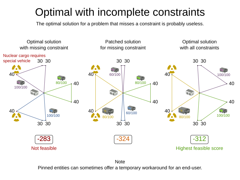
5.1.2. Formalize the business constraints
To implement a verbal business constraint, it needs to be formalized as a score constraint. Luckily, defining constraints in OptaPlanner is very flexible through the following score techniques:
-
Score signum (positive or negative): maximize or minimize a constraint type
-
Score weight: put a cost/profit on a constraint type
-
Score level (hard, soft, …): prioritize a group of constraint types
-
Pareto scoring (rarely used)
Take the time to acquaint yourself with the first three techniques. Once you understand them, formalizing most business constraints becomes straightforward.
|
Do not presume that your business knows all its score constraints in advance. Expect score constraints to be added, changed or removed after the first releases. |
5.1.3. Score constraint signum (positive or negative)
All score techniques are based on constraints. A constraint can be a simple pattern (such as Maximize the apple harvest in the solution) or a more complex pattern. A positive constraint is a constraint you want to maximize. A negative constraint is a constraint you want to minimize
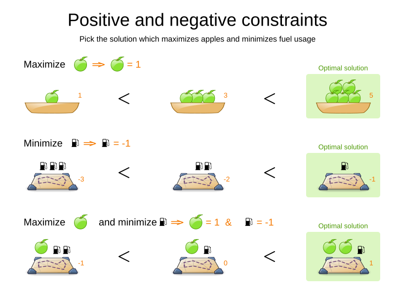
The image above illustrates that the optimal solution always has the highest score, regardless if the constraints are positive or negative.
Most planning problems have only negative constraints and therefore have a negative score. In that case, the score is the sum of the weight of the negative constraints being broken, with a perfect score of 0. For example in n queens, the score is the negative of the number of queen pairs which can attack each other.
Negative and positive constraints can be combined, even in the same score level.
When a constraint activates (because the negative constraint is broken or the positive constraint is fulfilled) on a certain planning entity set, it is called a constraint match.
5.1.4. Score constraint weight
Not all score constraints are equally important. If breaking one constraint is equally bad as breaking another constraint x times, then those two constraints have a different weight (but they are in the same score level). For example in vehicle routing, you can make one unhappy driver constraint match count as much as two fuel tank usage constraint matches:
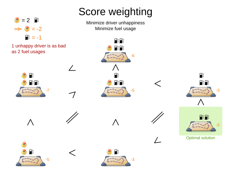
Score weighting is easy in use cases where you can put a price tag on everything. In that case, the positive constraints maximize revenue and the negative constraints minimize expenses, so together they maximize profit. Alternatively, score weighting is also often used to create social fairness. For example, a nurse, who requests a free day, pays a higher weight on New Years eve than on a normal day.
The weight of a constraint match can depend on the planning entities involved.
For example in cloud balancing, the weight of the soft constraint match for an active Computer
is the maintenance cost of that Computer (which differs per computer).
Putting a good weight on a constraint is often a difficult analytical decision, because it is about making choices and trade-offs against other constraints. Different stakeholders have different priorities. Don’t waste time with constraint weight discussions at the start of an implementation, instead add a constraint configuration and allow users to change them through a UI. A non-accurate weight is less damaging than mediocre algorithms:
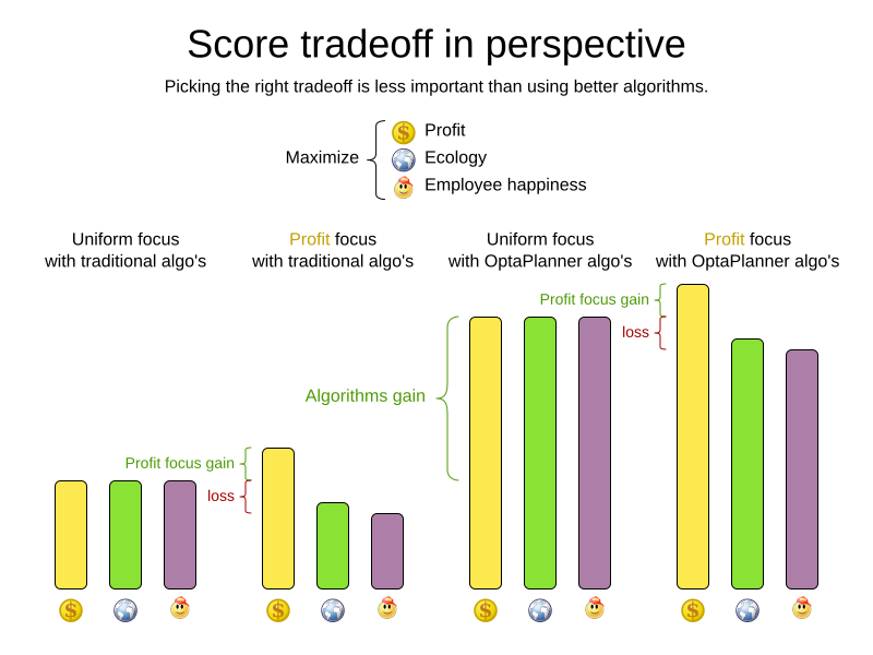
Most use cases use a Score with int weights, such as HardSoftScore.
5.1.5. Score constraint level (hard, soft, …)
Sometimes a score constraint outranks another score constraint, no matter how many times the latter is broken. In that case, those score constraints are in different levels. For example, a nurse cannot do two shifts at the same time (due to the constraints of physical reality), so this outranks all nurse happiness constraints.
Most use cases have only two score levels, hard and soft.
The levels of two scores are compared lexicographically.
The first score level gets compared first.
If those differ, the remaining score levels are ignored.
For example, a score that breaks 0 hard constraints and 1000000 soft constraints is better
than a score that breaks 1 hard constraint and 0 soft constraints.
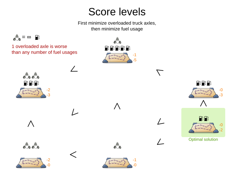
If there are two (or more) score levels, for example HardSoftScore, then a score is feasible if no hard constraints are broken.
|
By default, OptaPlanner will always assign all planning variables a planning value. If there is no feasible solution, this means the best solution will be infeasible. To instead leave some of the planning entities unassigned, apply overconstrained planning. |
For each constraint, you need to pick a score level, a score weight and a score signum.
For example: -1soft which has score level of soft, a weight of 1 and a negative signum.
Do not use a big constraint weight when your business actually wants different score levels.
That hack, known as score folding, is broken:
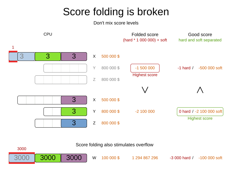
|
Your business might tell you that your hard constraints all have the same weight, because they cannot be broken (so the weight does not matter). This is not true because if no feasible solution exists for a specific dataset, the least infeasible solution allows the business to estimate how many business resources they are lacking. For example in cloud balancing, how many new computers to buy. Furthermore, it will likely create a score trap.
For example in cloud balance if a |
Three or more score levels are also supported. For example: a company might decide that profit outranks employee satisfaction (or vice versa), while both are outranked by the constraints of physical reality.
|
To model fairness or load balancing, there is no need to use lots of score levels (even though OptaPlanner can handle many score levels). |
Most use cases use a Score with two or three weights,
such as HardSoftScore and HardMediumSoftScore.
5.1.6. Pareto scoring (AKA multi-objective optimization scoring)
Far less common is the use case of pareto optimization, which is also known as multi-objective optimization. In pareto scoring, score constraints are in the same score level, yet they are not weighted against each other. When two scores are compared, each of the score constraints are compared individually and the score with the most dominating score constraints wins. Pareto scoring can even be combined with score levels and score constraint weighting.
Consider this example with positive constraints, where we want to get the most apples and oranges. Since it is impossible to compare apples and oranges, we cannot weigh them against each other. Yet, despite that we cannot compare them, we can state that two apples are better than one apple. Similarly, we can state that two apples and one orange are better than just one orange. So despite our inability to compare some Scores conclusively (at which point we declare them equal), we can find a set of optimal scores. Those are called pareto optimal.
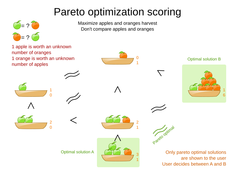
Scores are considered equal far more often. It is left up to a human to choose the better out of a set of best solutions (with equal scores) found by OptaPlanner. In the example above, the user must choose between solution A (three apples and one orange) and solution B (one apple and six oranges). It is guaranteed that OptaPlanner has not found another solution which has more apples or more oranges or even a better combination of both (such as two apples and three oranges).
Pareto scoring is currently not supported in OptaPlanner.
|
A pareto |
5.1.7. Combining score techniques
All the score techniques mentioned above, can be combined seamlessly:
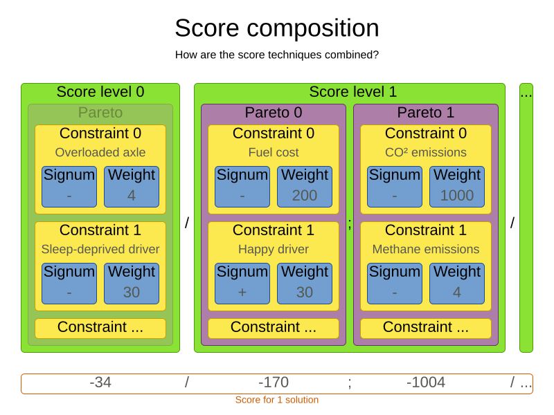
5.1.8. Score interface
A score is represented by the Score interface, which naturally extends Comparable:
public interface Score<...> extends Comparable<...> {
...
}The Score implementation to use depends on your use case.
Your score might not efficiently fit in a single long value.
OptaPlanner has several built-in Score implementations, but you can implement a custom Score too.
Most use cases tend to use the built-in HardSoftScore.
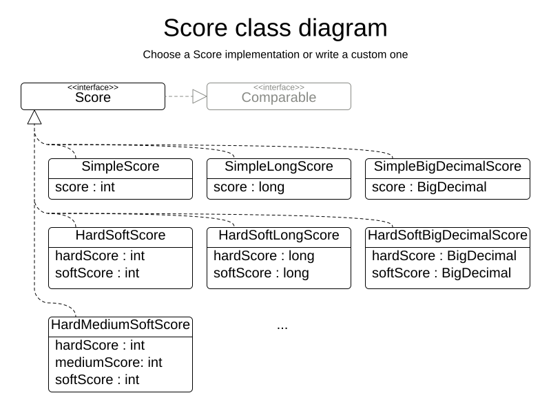
All Score implementations also have an initScore (which is an int).It is mostly intended for internal use in OptaPlanner: it is the negative number of uninitialized planning variables.
From a user’s perspective this is 0, unless a Construction Heuristic is terminated before it could initialize all planning variables (in which case Score.isSolutionInitialized() returns false).
The Score implementation (for example HardSoftScore) must be the same throughout a Solver runtime.
The Score implementation is configured in the solution domain class:
@PlanningSolution
public class CloudBalance {
...
@PlanningScore
private HardSoftScore score;
}5.1.9. Avoid floating point numbers in score calculation
Avoid the use of float or double in score calculation.
Use BigDecimal or scaled long instead.
Floating point numbers (float and double) cannot represent a decimal number correctly.
For example: a double cannot hold the value 0.05 correctly.
Instead, it holds the nearest representable value.
Arithmetic (including addition and subtraction) with floating point numbers, especially for planning problems, leads to incorrect decisions:
Additionally, floating point number addition is not associative:
System.out.println( ((0.01 + 0.02) + 0.03) == (0.01 + (0.02 + 0.03)) ); // returns falseThis leads to score corruption.
Decimal numbers (BigDecimal) have none of these problems.
|
BigDecimal arithmetic is considerably slower than Therefore, in many cases, it can be worthwhile to multiply all numbers for a single score weight by a plural of ten, so the score weight fits in a scaled |
5.2. Choose a score type
Depending on the number of score levels and type of score weights you need, choose a Score type.
Most use cases use a HardSoftScore.
|
To properly write a |
5.2.1. SimpleScore
A SimpleScore has a single int value, for example -123.
It has a single score level.
@PlanningScore
private SimpleScore score;Variants of this Score type:
-
SimpleLongScoreuses alongvalue instead of anintvalue. -
SimpleBigDecimalScoreuses aBigDecimalvalue instead of anintvalue.
5.2.2. HardSoftScore (Recommended)
A HardSoftScore has a hard int value and a soft int value, for example -123hard/-456soft.
It has two score levels (hard and soft).
@PlanningScore
private HardSoftScore score;Variants of this Score type:
-
HardSoftLongScoreuseslongvalues instead ofintvalues. -
HardSoftBigDecimalScoreusesBigDecimalvalues instead ofintvalues.
5.2.3. HardMediumSoftScore
A HardMediumSoftScore which has a hard int value, a medium int value and a soft int value, for example -123hard/-456medium/-789soft.
It has three score levels (hard, medium and soft).
The hard level determines if the solution is feasible,
and the medium level and soft level score values determine
how well the solution meets business goals.
Higher medium values take precedence over soft values irrespective of the soft value.
@PlanningScore
private HardMediumSoftScore score;Variants of this Score type:
-
HardMediumSoftLongScoreuseslongvalues instead ofintvalues. -
HardMediumSoftBigDecimalScoreusesBigDecimalvalues instead ofintvalues.
5.2.4. BendableScore
A BendableScore has a configurable number of score levels.
It has an array of hard int values and an array of soft int values,
for example with two hard levels and three soft levels, the score can be [-123/-456]hard/[-789/-012/-345]soft.
In that case, it has five score levels.
A solution is feasible if all hard levels are at least zero.
A BendableScore with one hard level and one soft level is equivalent to a HardSoftScore, while a BendableScore with one hard level and two soft levels is equivalent to a HardMediumSoftScore.
@PlanningScore(bendableHardLevelsSize = 2, bendableSoftLevelsSize = 3)
private BendableScore score;The number of hard and soft score levels need to be set at compilation time. It is not flexible to change during solving.
|
Do not use a Usually, multiple constraints share the same level and are weighted against each other. Use explaining the score to get the weight of individual constraints in the same level. |
Variants of this Score type:
-
BendableLongScoreuseslongvalues instead ofintvalues. -
BendableBigDecimalScoreusesBigDecimalvalues instead ofintvalues.
5.3. Calculate the Score
5.3.1. Score calculation types
There are several ways to calculate the Score of a solution:
-
Easy Java score calculation: Implement all constraints together in a single method in Java (or another JVM language). Does not scale.
-
Constraint streams score calculation: Implement each constraint as a separate Constraint Stream in Java (or another JVM language). Fast and scalable.
-
Incremental Java score calculation (not recommended): Implement multiple low-level methods in Java (or another JVM language). Fast and scalable. Very difficult to implement and maintain.
-
Drools score calculation (Deprecated): Implement each constraint as a separate score rule in DRL. Scalable.
Every score calculation type can work with any Score definition (such as HardSoftScore or HardMediumSoftScore).
All score calculation types are Object Oriented and can reuse existing Java code.
|
The score calculation must be read-only. It must not change the planning entities or the problem facts in any way. For example, it must not call a setter method on a planning entity in the score calculation. OptaPlanner does not recalculate the score of a solution if it can predict it (unless an environmentMode assertion is enabled). For example, after a winning step is done, there is no need to calculate the score because that move was done and undone earlier. As a result, there is no guarantee that changes applied during score calculation actually happen. To update planning entities when the planning variable change, use shadow variables instead. |
5.3.2. Easy Java score calculation
An easy way to implement your score calculation in Java.
-
Advantages:
-
Plain old Java: no learning curve
-
Opportunity to delegate score calculation to an existing code base or legacy system
-
-
Disadvantages:
-
Slower
-
Does not scale because there is no incremental score calculation
-
Implement the one method of the interface EasyScoreCalculator:
public interface EasyScoreCalculator<Solution_, Score_ extends Score<Score_>> {
Score_ calculateScore(Solution_ solution);
}For example in n queens:
public class NQueensEasyScoreCalculator
implements EasyScoreCalculator<NQueens, SimpleScore> {
@Override
public SimpleScore calculateScore(NQueens nQueens) {
int n = nQueens.getN();
List<Queen> queenList = nQueens.getQueenList();
int score = 0;
for (int i = 0; i < n; i++) {
for (int j = i + 1; j < n; j++) {
Queen leftQueen = queenList.get(i);
Queen rightQueen = queenList.get(j);
if (leftQueen.getRow() != null && rightQueen.getRow() != null) {
if (leftQueen.getRowIndex() == rightQueen.getRowIndex()) {
score--;
}
if (leftQueen.getAscendingDiagonalIndex() == rightQueen.getAscendingDiagonalIndex()) {
score--;
}
if (leftQueen.getDescendingDiagonalIndex() == rightQueen.getDescendingDiagonalIndex()) {
score--;
}
}
}
}
return SimpleScore.valueOf(score);
}
}Configure it in the solver configuration:
<scoreDirectorFactory>
<easyScoreCalculatorClass>org.optaplanner.examples.nqueens.optional.score.NQueensEasyScoreCalculator</easyScoreCalculatorClass>
</scoreDirectorFactory>To configure values of an EasyScoreCalculator dynamically in the solver configuration
(so the Benchmarker can tweak those parameters),
add the easyScoreCalculatorCustomProperties element and use custom properties:
<scoreDirectorFactory>
<easyScoreCalculatorClass>...MyEasyScoreCalculator</easyScoreCalculatorClass>
<easyScoreCalculatorCustomProperties>
<property name="myCacheSize" value="1000" />
</easyScoreCalculatorCustomProperties>
</scoreDirectorFactory>5.3.3. Incremental Java score calculation
A way to implement your score calculation incrementally in Java.
-
Advantages:
-
Very fast and scalable
-
Currently the fastest if implemented correctly
-
-
-
Disadvantages:
-
Hard to write
-
A scalable implementation heavily uses maps, indexes, … (things the Drools rule engine can do for you)
-
You have to learn, design, write and improve all these performance optimizations yourself
-
-
Hard to read
-
Regular score constraint changes can lead to a high maintenance cost
-
-
Implement all the methods of the interface IncrementalScoreCalculator:
public interface IncrementalScoreCalculator<Solution_, Score_ extends Score<Score_>> {
void resetWorkingSolution(Solution_ workingSolution);
void beforeEntityAdded(Object entity);
void afterEntityAdded(Object entity);
void beforeVariableChanged(Object entity, String variableName);
void afterVariableChanged(Object entity, String variableName);
void beforeEntityRemoved(Object entity);
void afterEntityRemoved(Object entity);
Score_ calculateScore();
}
For example in n queens:
public class NQueensAdvancedIncrementalScoreCalculator
implements IncrementalScoreCalculator<NQueens, SimpleScore> {
private Map<Integer, List<Queen>> rowIndexMap;
private Map<Integer, List<Queen>> ascendingDiagonalIndexMap;
private Map<Integer, List<Queen>> descendingDiagonalIndexMap;
private int score;
public void resetWorkingSolution(NQueens nQueens) {
int n = nQueens.getN();
rowIndexMap = new HashMap<Integer, List<Queen>>(n);
ascendingDiagonalIndexMap = new HashMap<Integer, List<Queen>>(n * 2);
descendingDiagonalIndexMap = new HashMap<Integer, List<Queen>>(n * 2);
for (int i = 0; i < n; i++) {
rowIndexMap.put(i, new ArrayList<Queen>(n));
ascendingDiagonalIndexMap.put(i, new ArrayList<Queen>(n));
descendingDiagonalIndexMap.put(i, new ArrayList<Queen>(n));
if (i != 0) {
ascendingDiagonalIndexMap.put(n - 1 + i, new ArrayList<Queen>(n));
descendingDiagonalIndexMap.put((-i), new ArrayList<Queen>(n));
}
}
score = 0;
for (Queen queen : nQueens.getQueenList()) {
insert(queen);
}
}
public void beforeEntityAdded(Object entity) {
// Do nothing
}
public void afterEntityAdded(Object entity) {
insert((Queen) entity);
}
public void beforeVariableChanged(Object entity, String variableName) {
retract((Queen) entity);
}
public void afterVariableChanged(Object entity, String variableName) {
insert((Queen) entity);
}
public void beforeEntityRemoved(Object entity) {
retract((Queen) entity);
}
public void afterEntityRemoved(Object entity) {
// Do nothing
}
private void insert(Queen queen) {
Row row = queen.getRow();
if (row != null) {
int rowIndex = queen.getRowIndex();
List<Queen> rowIndexList = rowIndexMap.get(rowIndex);
score -= rowIndexList.size();
rowIndexList.add(queen);
List<Queen> ascendingDiagonalIndexList = ascendingDiagonalIndexMap.get(queen.getAscendingDiagonalIndex());
score -= ascendingDiagonalIndexList.size();
ascendingDiagonalIndexList.add(queen);
List<Queen> descendingDiagonalIndexList = descendingDiagonalIndexMap.get(queen.getDescendingDiagonalIndex());
score -= descendingDiagonalIndexList.size();
descendingDiagonalIndexList.add(queen);
}
}
private void retract(Queen queen) {
Row row = queen.getRow();
if (row != null) {
List<Queen> rowIndexList = rowIndexMap.get(queen.getRowIndex());
rowIndexList.remove(queen);
score += rowIndexList.size();
List<Queen> ascendingDiagonalIndexList = ascendingDiagonalIndexMap.get(queen.getAscendingDiagonalIndex());
ascendingDiagonalIndexList.remove(queen);
score += ascendingDiagonalIndexList.size();
List<Queen> descendingDiagonalIndexList = descendingDiagonalIndexMap.get(queen.getDescendingDiagonalIndex());
descendingDiagonalIndexList.remove(queen);
score += descendingDiagonalIndexList.size();
}
}
public SimpleScore calculateScore() {
return SimpleScore.valueOf(score);
}
}Configure it in the solver configuration:
<scoreDirectorFactory>
<incrementalScoreCalculatorClass>org.optaplanner.examples.nqueens.optional.score.NQueensAdvancedIncrementalScoreCalculator</incrementalScoreCalculatorClass>
</scoreDirectorFactory>|
A piece of incremental score calculator code can be difficult to write and to review.
Assert its correctness by using an |
To configure values of an IncrementalScoreCalculator dynamically in the solver configuration
(so the Benchmarker can tweak those parameters),
add the incrementalScoreCalculatorCustomProperties element and use custom properties:
<scoreDirectorFactory>
<incrementalScoreCalculatorClass>...MyIncrementalScoreCalculator</incrementalScoreCalculatorClass>
<incrementalScoreCalculatorCustomProperties>
<property name="myCacheSize" value="1000"/>
</incrementalScoreCalculatorCustomProperties>
</scoreDirectorFactory>5.3.3.1. ConstraintMatchAwareIncrementalScoreCalculator
Optionally, also implement the ConstraintMatchAwareIncrementalScoreCalculator interface to:
-
Explain a score by splitting it up per score constraint with
ScoreExplanation.getConstraintMatchTotalMap(). -
Visualize or sort planning entities by how many constraints each one breaks with
ScoreExplanation.getIndictmentMap(). -
Receive a detailed analysis if the
IncrementalScoreCalculatoris corrupted inFAST_ASSERTorFULL_ASSERTenvironmentMode,
public interface ConstraintMatchAwareIncrementalScoreCalculator<Solution_, Score_ extends Score<Score_>> {
void resetWorkingSolution(Solution_ workingSolution, boolean constraintMatchEnabled);
Collection<ConstraintMatchTotal<Score_>> getConstraintMatchTotals();
Map<Object, Indictment<Score_>> getIndictmentMap();
}For example in machine reassignment, create one ConstraintMatchTotal per constraint type and call addConstraintMatch() for each constraint match:
public class MachineReassignmentIncrementalScoreCalculator
implements ConstraintMatchAwareIncrementalScoreCalculator<MachineReassignment, HardSoftLongScore> {
...
@Override
public void resetWorkingSolution(MachineReassignment workingSolution, boolean constraintMatchEnabled) {
resetWorkingSolution(workingSolution);
// ignore constraintMatchEnabled, it is always presumed enabled
}
@Override
public Collection<ConstraintMatchTotal<HardSoftLongScore>> getConstraintMatchTotals() {
ConstraintMatchTotal<HardSoftLongScore> maximumCapacityMatchTotal = new DefaultConstraintMatchTotal<>(CONSTRAINT_PACKAGE,
"maximumCapacity", HardSoftLongScore.ZERO);
...
for (MrMachineScorePart machineScorePart : machineScorePartMap.values()) {
for (MrMachineCapacityScorePart machineCapacityScorePart : machineScorePart.machineCapacityScorePartList) {
if (machineCapacityScorePart.maximumAvailable < 0L) {
maximumCapacityMatchTotal.addConstraintMatch(
Arrays.asList(machineCapacityScorePart.machineCapacity),
HardSoftLongScore.valueOf(machineCapacityScorePart.maximumAvailable, 0));
}
}
}
...
List<ConstraintMatchTotal<HardSoftLongScore>> constraintMatchTotalList = new ArrayList<>(4);
constraintMatchTotalList.add(maximumCapacityMatchTotal);
...
return constraintMatchTotalList;
}
@Override
public Map<Object, Indictment<HardSoftLongScore>> getIndictmentMap() {
return null; // Calculate it non-incrementally from getConstraintMatchTotals()
}
}That getConstraintMatchTotals() code often duplicates some of the logic of the normal IncrementalScoreCalculator methods.
Constraint Streams and Drools Score Calculation don’t have this disadvantage, because they are constraint match aware automatically when needed,
without any extra domain-specific code.
5.3.4. InitializingScoreTrend
The InitializingScoreTrend specifies how the Score will change as more and more variables are initialized (while the already initialized variables do not change). Some optimization algorithms (such Construction Heuristics and Exhaustive Search) run faster if they have such information.
For the Score (or each score level separately), specify a trend:
-
ANY(default): Initializing an extra variable can change the score positively or negatively. Gives no performance gain. -
ONLY_UP(rare): Initializing an extra variable can only change the score positively. Implies that:-
There are only positive constraints
-
And initializing the next variable cannot unmatch a positive constraint that was matched by a previous initialized variable.
-
-
ONLY_DOWN: Initializing an extra variable can only change the score negatively. Implies that:-
There are only negative constraints
-
And initializing the next variable cannot unmatch a negative constraint that was matched by a previous initialized variable.
-
Most use cases only have negative constraints.
Many of those have an InitializingScoreTrend that only goes down:
<scoreDirectorFactory>
<constraintProviderClass>org.optaplanner.examples.cloudbalancing.score.CloudBalancingConstraintProvider</constraintProviderClass>
<initializingScoreTrend>ONLY_DOWN</initializingScoreTrend>
</scoreDirectorFactory>Alternatively, you can also specify the trend for each score level separately:
<scoreDirectorFactory>
<constraintProviderClass>org.optaplanner.examples.cloudbalancing.score.CloudBalancingConstraintProvider</constraintProviderClass>
<initializingScoreTrend>ONLY_DOWN/ONLY_DOWN</initializingScoreTrend>
</scoreDirectorFactory>5.3.5. Invalid score detection
When you put the environmentMode in FULL_ASSERT (or FAST_ASSERT),
it will detect score corruption in the incremental score calculation.
However, that will not verify that your score calculator actually implements your score constraints as your business desires.
For example, one constraint might consistently match the wrong pattern.
To verify the constraints against an independent implementation, configure a assertionScoreDirectorFactory:
<environmentMode>FAST_ASSERT</environmentMode>
...
<scoreDirectorFactory>
<constraintProviderClass>org.optaplanner.examples.nqueens.optional.score.NQueensConstraintProvider</constraintProviderClass>
<assertionScoreDirectorFactory>
<easyScoreCalculatorClass>org.optaplanner.examples.nqueens.optional.score.NQueensEasyScoreCalculator</easyScoreCalculatorClass>
</assertionScoreDirectorFactory>
</scoreDirectorFactory>This way, the NQueensConstraintProvider implementation is validated by the EasyScoreCalculator.
|
This works well to isolate score corruption, but to verify that the constraint implement the real business needs, a unit test with a ConstraintVerifier is usually better. |
5.4. Score calculation performance tricks
5.4.1. Overview
The Solver will normally spend most of its execution time running the score calculation
(which is called in its deepest loops).
Faster score calculation will return the same solution in less time with the same algorithm,
which normally means a better solution in equal time.
5.4.2. Score calculation speed
After solving a problem, the Solver will log the score calculation speed per second.
This is a good measurement of Score calculation performance,
despite that it is affected by non score calculation execution time.
It depends on the problem scale of the problem dataset.
Normally, even for high scale problems, it is higher than 1000, except if you are using an EasyScoreCalculator.
|
When improving your score calculation, focus on maximizing the score calculation speed, instead of maximizing the best score. A big improvement in score calculation can sometimes yield little or no best score improvement, for example when the algorithm is stuck in a local or global optima. If you are watching the calculation speed instead, score calculation improvements are far more visible. Furthermore, watching the calculation speed allows you to remove or add score constraints, and still compare it with the original’s calculation speed. Comparing the best score with the original’s best score is pointless: it’s comparing apples and oranges. |
5.4.3. Incremental score calculation (with deltas)
When a solution changes, incremental score calculation (AKA delta based score calculation)
calculates the delta with the previous state to find the new Score,
instead of recalculating the entire score on every solution evaluation.
For example, when a single queen A moves from row 1 to 2,
it will not bother to check if queen B and C can attack each other, since neither of them changed:
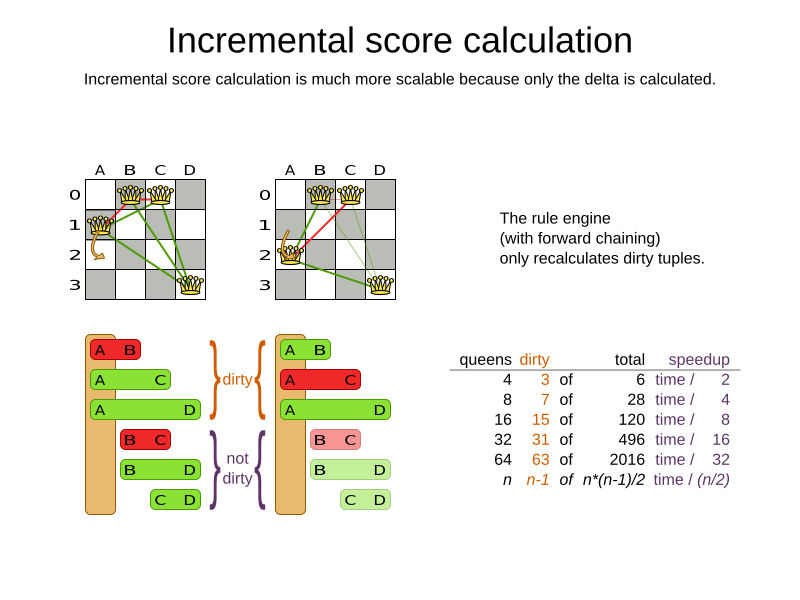
Similarly in employee rostering:
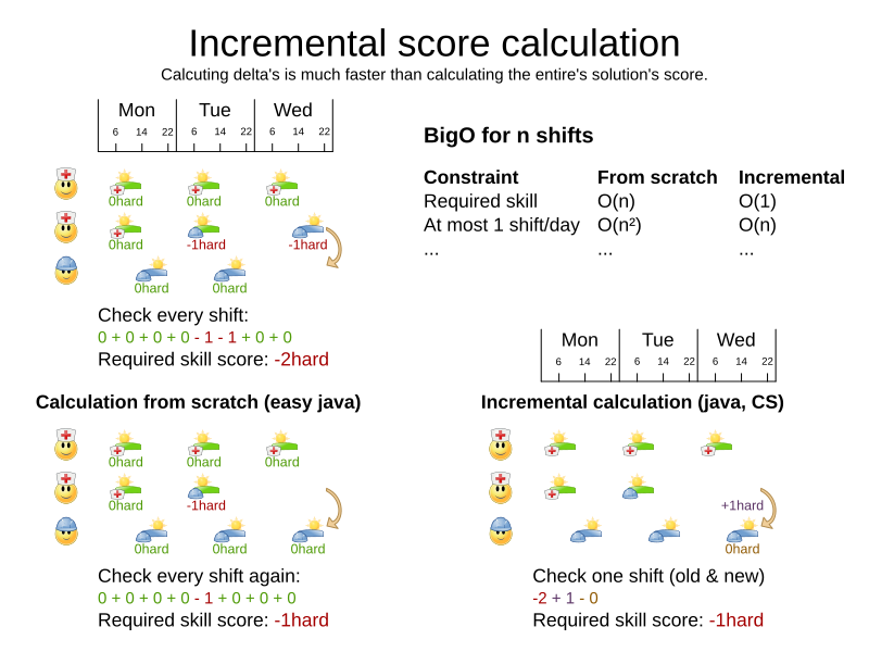
This is a huge performance and scalability gain. Constraint Streams or Drools score calculation give you this huge scalability gain without forcing you to write a complicated incremental score calculation algorithm. Just let the rule engine do the hard work.
Notice that the speedup is relative to the size of your planning problem (your n), making incremental score calculation far more scalable.
5.4.4. Avoid calling remote services during score calculation
Do not call remote services in your score calculation (except if you are bridging EasyScoreCalculator to a legacy system). The network latency will kill your score calculation performance.
Cache the results of those remote services if possible.
If some parts of a constraint can be calculated once, when the Solver starts, and never change during solving,
then turn them into cached problem facts.
5.4.5. Pointless constraints
If you know a certain constraint can never be broken (or it is always broken), do not write a score constraint for it.
For example in n queens, the score calculation does not check if multiple queens occupy the same column,
because a Queen's column never changes and every solution starts with each Queen on a different column.
|
Do not go overboard with this. If some datasets do not use a specific constraint but others do, just return out of the constraint as soon as you can. There is no need to dynamically change your score calculation based on the dataset. |
5.4.6. Built-in hard constraint
Instead of implementing a hard constraint, it can sometimes be built in.
For example, if Lecture A should never be assigned to Room X, but it uses ValueRangeProvider on Solution,
so the Solver will often try to assign it to Room X too (only to find out that it breaks a hard constraint).
Use a ValueRangeProvider on the planning entity or filtered selection to define that Course A should only be assigned a Room different than X.
This can give a good performance gain in some use cases, not just because the score calculation is faster, but mainly because most optimization algorithms will spend less time evaluating infeasible solutions. However, usually this is not a good idea because there is a real risk of trading short term benefits for long term harm:
-
Many optimization algorithms rely on the freedom to break hard constraints when changing planning entities, to get out of local optima.
-
Both implementation approaches have limitations (feature compatibility, disabling automatic performance optimizations), as explained in their documentation.
5.4.7. Other score calculation performance tricks
-
Verify that your score calculation happens in the correct
Numbertype. If you are making the sum ofintvalues, do not sum it in adoublewhich takes longer. -
For optimal performance, always use server mode (
java -server). We have seen performance increases of 50% by turning on server mode. -
For optimal performance, use the latest Java version. For example, in the past we have seen performance increases of 30% by switching from java 1.5 to 1.6.
-
Always remember that premature optimization is the root of all evil. Make sure your design is flexible enough to allow configuration based tweaking.
5.4.8. Score trap
Make sure that none of your score constraints cause a score trap. A trapped score constraint uses the same weight for different constraint matches, when it could just as easily use a different weight. It effectively lumps its constraint matches together, which creates a flatlined score function for that constraint. This can cause a solution state in which several moves need to be done to resolve or lower the weight of that single constraint. Some examples of score traps:
-
You need two doctors at each table, but you are only moving one doctor at a time. So the solver has no incentive to move a doctor to a table with no doctors. Punish a table with no doctors more than a table with only one doctor in that score constraint in the score function.
-
Two exams need to be conducted at the same time, but you are only moving one exam at a time. So the solver has to move one of those exams to another timeslot without moving the other in the same move. Add a coarse-grained move that moves both exams at the same time.
For example, consider this score trap. If the blue item moves from an overloaded computer to an empty computer, the hard score should improve. The trapped score implementation fails to do that:
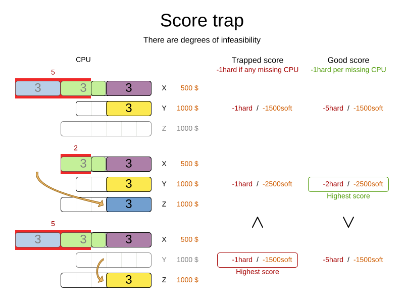
The Solver should eventually get out of this trap, but it will take a lot of effort (especially if there are even more processes on the overloaded computer). Before they do that, they might actually start moving more processes into that overloaded computer, as there is no penalty for doing so.
|
Avoiding score traps does not mean that your score function should be smart enough to avoid local optima. Leave it to the optimization algorithms to deal with the local optima. Avoiding score traps means to avoid, for each score constraint individually, a flatlined score function. |
|
Always specify the degree of infeasibility. The business will often say "if the solution is infeasible, it does not matter how infeasible it is." While that is true for the business, it is not true for score calculation as it benefits from knowing how infeasible it is. In practice, soft constraints usually do this naturally and it is just a matter of doing it for the hard constraints too. |
There are several ways to deal with a score trap:
-
Improve the score constraint to make a distinction in the score weight. For example, penalize
-1hardfor every missing CPU, instead of just-1hardif any CPU is missing. -
If changing the score constraint is not allowed from the business perspective, add a lower score level with a score constraint that makes such a distinction. For example, penalize
-1subsoftfor every missing CPU, on top of-1hardif any CPU is missing. The business ignores the subsoft score level. -
Add coarse-grained moves and union select them with the existing fine-grained moves. A coarse-grained move effectively does multiple moves to directly get out of a score trap with a single move. For example, move multiple items from the same container to another container.
5.4.9. stepLimit benchmark
Not all score constraints have the same performance cost. Sometimes one score constraint can kill the score calculation performance outright. Use the Benchmarker to do a one minute run and check what happens to the score calculation speed if you comment out all but one of the score constraints.
5.4.10. Fairness score constraints
Some use cases have a business requirement to provide a fair schedule (usually as a soft score constraint), for example:
-
Fairly distribute the workload amongst the employees, to avoid envy.
-
Evenly distribute the workload amongst assets, to improve reliability.
Implementing such a constraint can seem difficult (especially because there are different ways to formalize fairness), but usually the squared workload implementation behaves most desirable.
For each employee/asset, count the workload w and subtract w² from the score.
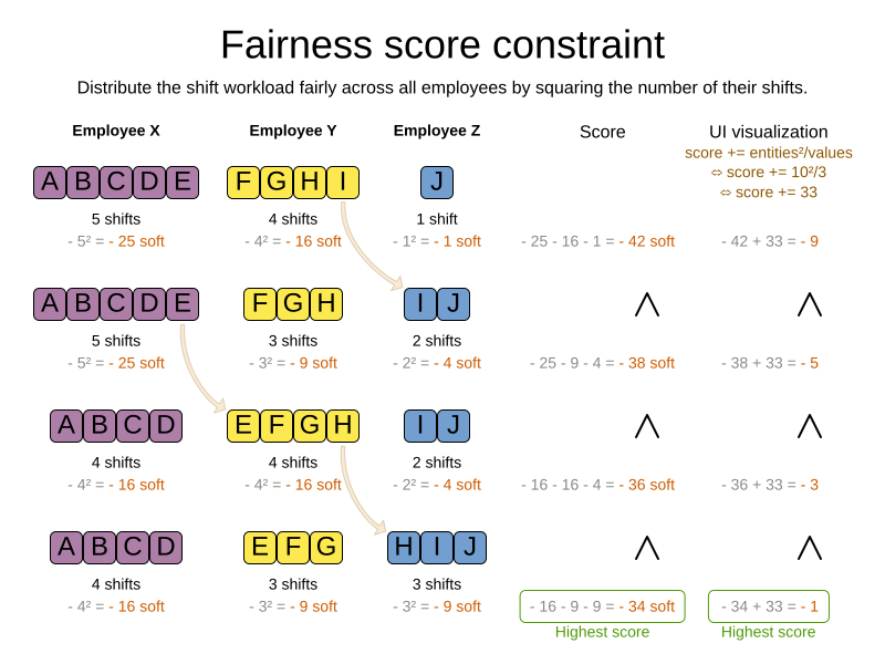
As shown above, the squared workload implementation guarantees that if you select two employees from a given solution and make their distribution between those two employees fairer, then the resulting new solution will have a better overall score. Do not just use the difference from the average workload, as that can lead to unfairness, as demonstrated below.
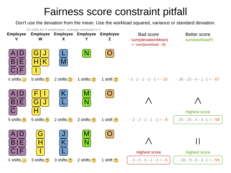
|
Instead of the squared workload, it is also possible to use the variance (squared difference to the average) or the standard deviation (square root of the variance). This has no effect on the score comparison, because the average will not change during planning. It is just more work to implement (because the average needs to be known) and trivially slower (because the calculation is a bit longer). |
When the workload is perfectly balanced, the user often likes to see a 0 score, instead of the distracting -34soft in the image above (for the last solution which is almost perfectly balanced).
To nullify this, either add the average multiplied by the number of entities to the score or instead show the variance or standard deviation in the UI.
5.5. Constraint configuration: adjust constraint weights dynamically
Deciding the correct weight and level for each constraint is not easy. It often involves negotiating with different stakeholders and their priorities. Furthermore, quantifying the impact of soft constraints is often a new experience for business managers, so they’ll need a number of iterations to get it right.
Don’t get stuck between a rock and a hard place. Provide a UI to adjust the constraint weights and visualize the resulting solution, so the business managers can tweak the constraint weights themselves:
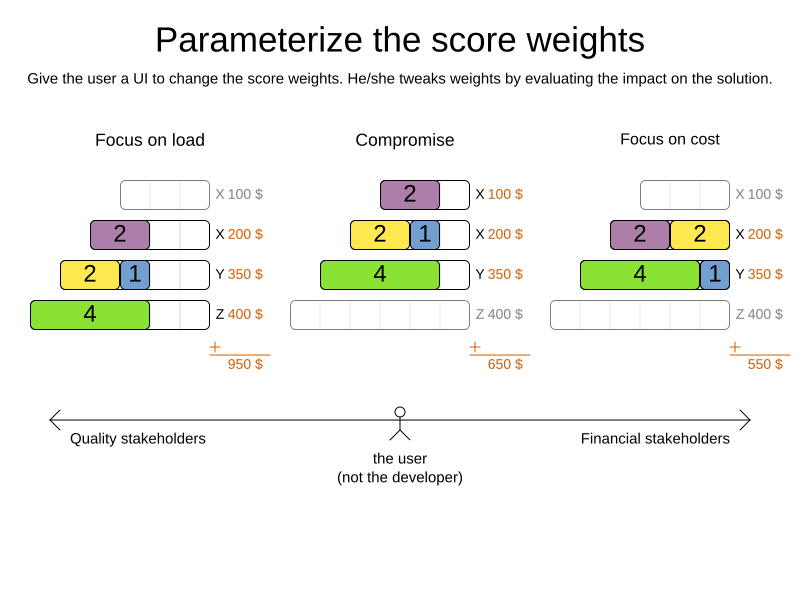
5.5.1. Create a constraint configuration
First, create a new class to hold the constraint weights and other constraint parameters.
Annotate it with @ConstraintConfiguration:
@ConstraintConfiguration
public class ConferenceConstraintConfiguration {
...
}There will be exactly one instance of this class per planning solution.
The planning solution and the constraint configuration have a one-to-one relationship,
but they serve a different purpose, so they aren’t merged into a single class.
A @ConstraintConfiguration class can extend a parent @ConstraintConfiguration class,
which can be useful in international use cases with many regional constraints.
Add the constraint configuration on the planning solution
and annotate that field or property with @ConstraintConfigurationProvider:
@PlanningSolution
public class ConferenceSolution {
@ConstraintConfigurationProvider
private ConferenceConstraintConfiguration constraintConfiguration;
...
}The @ConstraintConfigurationProvider annotation automatically exposes the constraint configuration
as a problem fact, there is no need to add a @ProblemFactProperty annotation.
The constraint configuration class holds the constraint weights,
but it can also hold constraint parameters.
For example in conference scheduling, the minimum pause constraint has a constraint weight (like any other constraint),
but it also has a constraint parameter that defines the length of the minimum pause between two talks of the same speaker.
That pause length depends on the conference (= the planning problem):
in some big conferences 20 minutes isn’t enough to go from one room to the other.
That pause length is a field in the constraint configuration without a @ConstraintWeight annotation.
5.5.2. Add a constraint weight for each constraint
In the constraint configuration class, add a @ConstraintWeight field or property for each constraint:
@ConstraintConfiguration(constraintPackage = "...conferencescheduling.score")
public class ConferenceConstraintConfiguration {
@ConstraintWeight("Speaker conflict")
private HardMediumSoftScore speakerConflict = HardMediumSoftScore.ofHard(10);
@ConstraintWeight("Theme track conflict")
private HardMediumSoftScore themeTrackConflict = HardMediumSoftScore.ofSoft(10);
@ConstraintWeight("Content conflict")
private HardMediumSoftScore contentConflict = HardMediumSoftScore.ofSoft(100);
...
}The type of the constraint weights must be the same score class as the planning solution’s score member.
For example in conference scheduling, ConferenceSolution.getScore() and ConferenceConstraintConfiguration.getSpeakerConflict()
both return a HardMediumSoftScore.
A constraint weight cannot be null.
Give each constraint weight a default value, but expose them in a UI so the business users can tweak them.
The example above uses the ofHard(), ofMedium() and ofSoft() methods to do that.
Notice how it defaults the content conflict constraint as ten times more important than the theme track conflict constraint.
Normally, a constraint weight only uses one score level,
but it’s possible to use multiple score levels (at a small performance cost).
Each constraint has a constraint package and a constraint name, together they form the constraint id. These connect the constraint weight with the constraint implementation. For each constraint weight, there must be a constraint implementation with the same package and the same name.
-
The
@ConstraintConfigurationannotation has aconstraintPackageproperty that defaults to the package of the constraint configuration class. Cases with Constraint streams normally don’t need to specify it. Cases with Drools score calculation (Deprecated) may need to override that because the DRLs often use a different package. -
The
@ConstraintWeightannotation has avaluewhich is the constraint name (for example "Speaker conflict"). It inherits the constraint package from the@ConstraintConfiguration, but it can override that, for example@ConstraintWeight(constraintPackage = "…region.france", …)to use a different constraint package than some other weights.
So every constraint weight ends up with a constraint package and a constraint name. Each constraint weight links with a constraint implementation, for example in Constraint Streams:
public final class ConferenceSchedulingConstraintProvider implements ConstraintProvider {
@Override
public Constraint[] defineConstraints(ConstraintFactory factory) {
return new Constraint[] {
speakerConflict(factory),
themeTrackConflict(factory),
contentConflict(factory),
...
};
}
protected Constraint speakerConflict(ConstraintFactory factory) {
return factory.forEachUniquePair(...)
...
.penalizeConfigurable("Speaker conflict", ...);
}
protected Constraint themeTrackConflict(ConstraintFactory factory) {
return factory.forEachUniquePair(...)
...
.penalizeConfigurable("Theme track conflict", ...);
}
protected Constraint contentConflict(ConstraintFactory factory) {
return factory.forEachUniquePair(...)
...
.penalizeConfigurable("Content conflict", ...);
}
...
}Each of the constraint weights defines the score level and score weight of their constraint.
The constraint implementation calls rewardConfigurable() or penalizeConfigurable() and the constraint weight is automatically applied.
If the constraint implementation provides a match weight, that match weight is multiplied with the constraint weight.
For example, the content conflict constraint weight defaults to 100soft
and the constraint implementation penalizes each match based on the number of shared content tags and the overlapping duration of the two talks:
@ConstraintWeight("Content conflict")
private HardMediumSoftScore contentConflict = HardMediumSoftScore.ofSoft(100);Constraint contentConflict(ConstraintFactory factory) {
return factory.forEachUniquePair(Talk.class,
overlapping(t -> t.getTimeslot().getStartDateTime(),
t -> t.getTimeslot().getEndDateTime()),
filtering((talk1, talk2) -> talk1.overlappingContentCount(talk2) > 0))
.penalizeConfigurable("Content conflict",
(talk1, talk2) -> talk1.overlappingContentCount(talk2)
* talk1.overlappingDurationInMinutes(talk2));
}So when 2 overlapping talks share only 1 content tag and overlap by 60 minutes, the score is impacted by -6000soft.
But when 2 overlapping talks share 3 content tags, the match weight is 180, so the score is impacted by -18000soft.
5.6. Explaining the score: which constraints are broken?
The easiest way to explain the score during development is to print the return value of getSummary(), but only use that method for diagnostic purposes:
System.out.println(scoreManager.getSummary(solution));For example in conference scheduling, this prints that talk S51 is responsible for breaking the hard constraint Speaker required room tag:
Explanation of score (-1hard/-806soft):
Constraint match totals:
-1hard: constraint (Speaker required room tag) has 1 matches:
-1hard: justifications ([S51])
-340soft: constraint (Theme track conflict) has 32 matches:
-20soft: justifications ([S68, S66])
-20soft: justifications ([S61, S44])
...
...
Indictments (top 5 of 72):
-1hard/-22soft: justification (S51) has 12 matches:
-1hard: constraint (Speaker required room tag)
-10soft: constraint (Theme track conflict)
...
...
|
Do not attempt to parse this string or use it in your UI or exposed services. Instead use the ConstraintMatch API below and do it properly. |
In the string above, there are two previously unexplained concepts.
Justifications are user-defined objects that implement the org.optaplanner.core.api.score.stream.ConstraintJustification interface,
which carry meaningful information about a constraint match, such as its package, name and score.
On the other hand, indicted objects are objects which were directly involved in causing a constraint to match. For example, if your constraints penalize each vehicle, then there will be one org.optaplanner.core.api.score.constraint.Indictment instance per vehicle, carrying the vehicle as an indicted object. Indictments are typically used for heat map visualization.
5.6.1. Using score calculation outside the Solver
If other parts of your application, for example your webUI, need to calculate the score of a solution, use the SolutionManager API:
SolutionManager<CloudBalance, HardSoftScore> scoreManager = SolutionManager.create(solverFactory);
ScoreExplanation<CloudBalance, HardSoftScore> scoreExplanation = scoreManager.explainScore(cloudBalance);Then use it when you need to calculate the Score of a solution:
HardSoftScore score = scoreExplanation.getScore();Furthermore, the ScoreExplanation can help explain the score through constraint match totals and/or indictments:
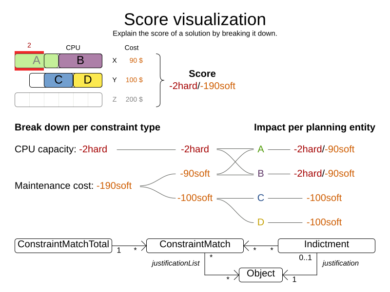
5.6.2. Break down the score by constraint justification
Each constraint may be justified by a different ConstraintJustification implementation, but you can also choose to share them among constraints.
To receive all constraint justifications regardless of their type, call:
List<ConstraintJustification> constraintJustificationlist = scoreExplanation.getJustificationList();
...In score DRL, justifications are always instances of
org.optaplanner.core.api.score.stream.DefaultConstraintJustification,
while in constraint streams, the return type can be customised,
so that it can be easily serialized and sent over the wire.
Such custom justifications can be queried like so:
List<MyConstraintJustification> constraintJustificationlist = scoreExplanation.getJustificationList(MyConstraintJustification.class);
...5.6.3. Break down the score by constraint
To break down the score per constraint, get the ConstraintMatchTotals from the ScoreExplanation:
Collection<ConstraintMatchTotal<HardSoftScore>> constraintMatchTotals = scoreExplanation.getConstraintMatchTotalMap().values();
for (ConstraintMatchTotal<HardSoftScore> constraintMatchTotal : constraintMatchTotals) {
String constraintName = constraintMatchTotal.getConstraintName();
// The score impact of that constraint
HardSoftScore totalScore = constraintMatchTotal.getScore();
for (ConstraintMatch<HardSoftScore> constraintMatch : constraintMatchTotal.getConstraintMatchSet()) {
ConstraintJustification justification = constraintMatch.getJustification();
HardSoftScore score = constraintMatch.getScore();
...
}
}Each ConstraintMatchTotal represents one constraint and has a part of the overall score.
The sum of all the ConstraintMatchTotal.getScore() equals the overall score.
|
Constraint streams and Drools score calculation supports constraint matches automatically, but incremental Java score calculation requires implementing an extra interface. |
5.6.4. Indictment heat map: visualize the hot planning entities
To show a heat map in the UI that highlights the planning entities and problem facts have an impact on the Score, get the Indictment map from the ScoreExplanation:
Map<Object, Indictment<HardSoftScore>> indictmentMap = scoreExplanation.getIndictmentMap();
for (CloudProcess process : cloudBalance.getProcessList()) {
Indictment<HardSoftScore> indictment = indictmentMap.get(process);
if (indictment == null) {
continue;
}
// The score impact of that planning entity
HardSoftScore totalScore = indictment.getScore();
for (ConstraintMatch<HardSoftScore> constraintMatch : indictment.getConstraintMatchSet()) {
String constraintName = constraintMatch.getConstraintName();
HardSoftScore score = constraintMatch.getScore();
...
}
}Each Indictment is the sum of all constraints where that justification object is involved with.
The sum of all the Indictment.getScoreTotal() differs from the overall score, because multiple Indictments can share the same ConstraintMatch.
|
Constraint streams and Drools score calculation supports constraint matches automatically, but incremental Java score calculation requires implementing an extra interface. |
5.7. Testing score constraints
It’s recommended to write a unit test for each score constraint individually to check that it behaves correctly. Different score calculation types come with different tools for testing. For more, see testing Constraint Streams or testing Drools constraints.
6. Constraint streams score calculation
Constraint streams are a Functional Programming form of incremental score calculation in plain Java that is easy to read, write and debug. The API should feel familiar if you’re familiar with Java Streams or SQL.
6.1. Introduction
Using Java’s Streams API, we could implement an easy score calculator that uses a functional approach:
private int doNotAssignAnn() {
int softScore = 0;
schedule.getShiftList().stream()
.filter(Shift::isEmployeeAnn)
.forEach(shift -> {
softScore -= 1;
});
return softScore;
}However, that scales poorly because it doesn’t do an incremental calculation:
When the planning variable of a single Shift changes, to recalculate the score,
the normal Streams API has to execute the entire stream from scratch.
The ConstraintStreams API enables you to write similar code in pure Java, while reaping the performance benefits of
incremental score calculation.
This is an example of the same code, using the Constraint Streams API:
private Constraint doNotAssignAnn(ConstraintFactory factory) {
return factory.forEach(Shift.class)
.filter(Shift::isEmployeeAnn)
.penalize(HardSoftScore.ONE_SOFT)
.asConstraint("Don't assign Ann");
}This constraint stream iterates over all instances of class Shift in the problem facts and
planning entities in the planning problem.
It finds every Shift which is assigned to employee Ann and for every such instance (also called a match), it adds a
soft penalty of 1 to the overall score.
The following figure illustrates this process on a problem with 4 different shifts:
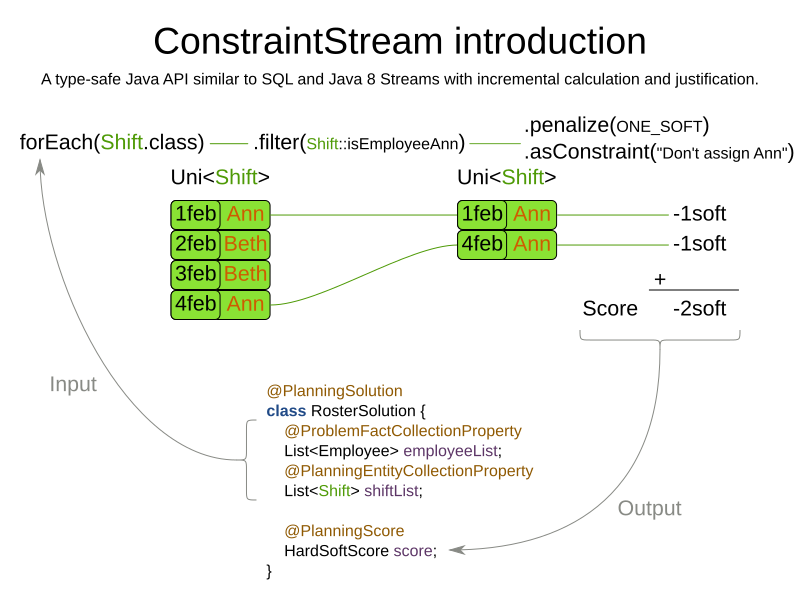
If any of the instances change during solving, the constraint stream automatically detects the change and only recalculates the minimum necessary portion of the problem that is affected by the change. The following figure illustrates this incremental score calculation:
ConstraintStreams API also has advanced support for score explanation through custom justifications and indictments.
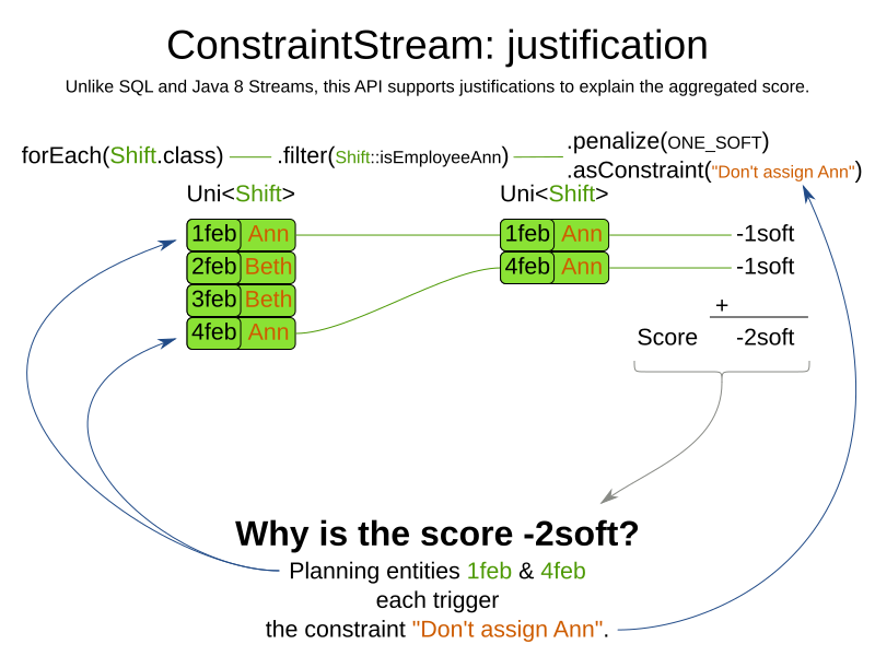
6.2. Creating a constraint stream
To use the ConstraintStreams API in your project, first write a pure Java ConstraintProvider implementation similar
to the following example.
public class MyConstraintProvider implements ConstraintProvider {
@Override
public Constraint[] defineConstraints(ConstraintFactory factory) {
return new Constraint[] {
penalizeEveryShift(factory)
};
}
private Constraint penalizeEveryShift(ConstraintFactory factory) {
return factory.forEach(Shift.class)
.penalize(HardSoftScore.ONE_SOFT)
.asConstraint("Penalize a shift");
}
}|
This example contains one constraint, |
Add the following code to your solver configuration:
<solver xmlns="https://www.optaplanner.org/xsd/solver" xmlns:xsi="http://www.w3.org/2001/XMLSchema-instance"
xsi:schemaLocation="https://www.optaplanner.org/xsd/solver https://www.optaplanner.org/xsd/solver/solver.xsd">
<scoreDirectorFactory>
<constraintProviderClass>org.acme.schooltimetabling.solver.TimeTableConstraintProvider</constraintProviderClass>
</scoreDirectorFactory>
...
</solver>6.3. Constraint stream cardinality
Constraint stream cardinality is a measure of how many objects a single constraint match consists of.
The simplest constraint stream has a cardinality of 1, meaning each constraint match only consists of 1 object.
Therefore, it is called a UniConstraintStream:
private Constraint doNotAssignAnn(ConstraintFactory factory) {
return factory.forEach(Shift.class) // Returns UniStream<Shift>.
...
}Some constraint stream building blocks can increase stream cardinality, such as join or groupBy:
private Constraint doNotAssignAnn(ConstraintFactory factory) {
return factory.forEach(Shift.class) // Returns Uni<Shift>.
.join(Employee.class) // Returns Bi<Shift, Employee>.
.join(DayOff.class) // Returns Tri<Shift, Employee, DayOff>.
.join(Country.class) // Returns Quad<Shift, Employee, DayOff, Country>.
...
}The latter can also decrease stream cardinality:
private Constraint doNotAssignAnn(ConstraintFactory factory) {
return factory.forEach(Shift.class) // Returns UniStream<Shift>.
.join(Employee.class) // Returns BiStream<Shift, Employee>.
.groupBy((shift, employee) -> employee) // Returns UniStream<Employee>.
...
}The following constraint stream cardinalities are currently supported:
Cardinality |
Prefix |
Defining interface |
1 |
Uni |
|
2 |
Bi |
|
3 |
Tri |
|
4 |
Quad |
|
6.3.1. Achieving higher cardinalities
OptaPlanner currently does not support constraint stream cardinalities higher than 4. However, with tuple mapping effectively infinite cardinality is possible:
private Constraint pentaStreamExample(ConstraintFactory factory) {
return factory.forEach(Shift.class) // UniConstraintStream<Shift>
.join(Shift.class) // BiConstraintStream<Shift, Shift>
.join(Shift.class) // TriConstraintStream<Shift, Shift, Shift>
.join(Shift.class) // QuadConstraintStream<Shift, Shift, Shift, Shift>
.map(MyTuple::of) // UniConstraintStream<MyTuple<Shift, Shift, Shift, Shift>>
.join(Shift.class) // BiConstraintStream<MyTuple<Shift, Shift, Shift, Shift>, Shift>
... // This BiConstraintStream carries 5 Shift elements.
}|
OptaPlanner does not provide any tuple implementations out of the box. It’s recommended to use one of the freely available 3rd party implementations. Should a custom implementation be necessary, see guidelines for mapping functions. |
6.4. Building blocks
Constraint streams are chains of different operations, called building blocks.
Each constraint stream starts with a forEach(…) building block and is terminated by either a penalty or a reward.
The following example shows the simplest possible constraint stream:
private Constraint penalizeInitializedShifts(ConstraintFactory factory) {
return factory.forEach(Shift.class)
.penalize(HardSoftScore.ONE_SOFT)
.asConstraint("Initialized shift");
}This constraint stream penalizes each known and initialized instance of Shift.
6.4.1. ForEach
The .forEach(T) building block selects every T instance that
is in a problem fact collection
or a planning entity collection
and has no null genuine planning variables.
To include instances with a null genuine planning variable,
replace the forEach() building block by forEachIncludingNullVars():
private Constraint penalizeAllShifts(ConstraintFactory factory) {
return factory.forEachIncludingNullVars(Shift.class)
.penalize(HardSoftScore.ONE_SOFT)
.asConstraint("A shift");
}|
The |
6.4.2. Penalties and rewards
The purpose of constraint streams is to build up a score for a solution.
To do this, every constraint stream must contain a call to either a penalize() or a reward()
building block.
The penalize() building block makes the score worse and the reward() building block improves the score.
Each constraint stream is then terminated by calling asConstraint() method, which finally builds the constraint. Constraints have several components:
-
Constraint package is the Java package that contains the constraint. The default value is the package that contains the
ConstraintProviderimplementation or the value from constraint configuration, if implemented. -
Constraint name is the human-readable descriptive name for the constraint, which (together with the constraint package) must be unique within the entire
ConstraintProviderimplementation. -
Constraint weight is a constant score value indicating how much every breach of the constraint affects the score. Valid examples include
SimpleScore.ONE,HardSoftScore.ONE_HARDandHardMediumSoftScore.of(1, 2, 3). -
Constraint match weigher is an optional function indicating how many times the constraint weight should be applied in the score. The penalty or reward score impact is the constraint weight multiplied by the match weight. The default value is
1.
|
Constraints with zero constraint weight are automatically disabled and do not impose any performance penalty. |
The ConstraintStreams API supports many different types of penalties. Browse the API in your IDE for the full list of method overloads. Here are some examples:
-
Simple penalty (
penalize(SimpleScore.ONE)) makes the score worse by1per every match in the constraint stream. The score type must be the same type as used on the@PlanningScoreannotated member on the planning solution. -
Dynamic penalty (
penalize(SimpleScore.ONE, Shift::getHours)) makes the score worse by the number of hours in every matchingShiftin the constraint stream. This is an example of using a constraint match weigher. -
Configurable penalty (
penalizeConfigurable()) makes the score worse using constraint weights defined in constraint configuration. -
Configurable dynamic penalty(
penalizeConfigurable(Shift::getHours)) makes the score worse using constraint weights defined in constraint configuration, multiplied by the number of hours in every matchingShiftin the constraint stream.
By replacing the keyword penalize by reward in the name of these building blocks, you get operations that
affect score in the opposite direction.
6.4.2.1. Customizing justifications and indictments
One of important OptaPlanner features is its ability to explain the score of solutions it produced through the use of justifications and indictments.
By default, each constraint is justified with org.optaplanner.core.api.score.stream.DefaultConstraintJustification, and the final tuple makes up the indicted objects.
For example, in the following constraint, the indicted objects will be of type Vehicle and an Integer:
protected Constraint vehicleCapacity(ConstraintFactory factory) {
return factory.forEach(Customer.class)
.filter(customer -> customer.getVehicle() != null)
.groupBy(Customer::getVehicle, sum(Customer::getDemand))
.filter((vehicle, demand) -> demand > vehicle.getCapacity())
.penalizeLong(HardSoftLongScore.ONE_HARD,
(vehicle, demand) -> demand - vehicle.getCapacity())
.asConstraint("vehicleCapacity");
}For the purposes of creating a heat map, the Vehicle is very important, but the naked Integer carries no semantics.
We can remove it by providing the `indictWith(…) method with a custom indictment mapping:
protected Constraint vehicleCapacity(ConstraintFactory factory) {
return factory.forEach(Customer.class)
.filter(customer -> customer.getVehicle() != null)
.groupBy(Customer::getVehicle, sum(Customer::getDemand))
.filter((vehicle, demand) -> demand > vehicle.getCapacity())
.penalizeLong(HardSoftLongScore.ONE_HARD,
(vehicle, demand) -> demand - vehicle.getCapacity())
.indictWith((vehicle, demand) -> List.of(vehicle))
.asConstraint("vehicleCapacity");
}The same mechanism can also be used to transform any of the indicted objects to any other object.
To present the constraint matches to the user or to send them over the wire where they can be further processed, use the justifyWith(…) method to provide a custom constraint justification:
protected Constraint vehicleCapacity(ConstraintFactory factory) {
return factory.forEach(Customer.class)
.filter(customer -> customer.getVehicle() != null)
.groupBy(Customer::getVehicle, sum(Customer::getDemand))
.filter((vehicle, demand) -> demand > vehicle.getCapacity())
.penalizeLong(HardSoftLongScore.ONE_HARD,
(vehicle, demand) -> demand - vehicle.getCapacity())
.justifyWith((vehicle, demand, score) ->
new VehicleDemandOveruse(vehicle, demand, score))
.indictWith((vehicle, demand) -> List.of(vehicle))
.asConstraint("vehicleCapacity");
}VehicleDemandOveruse is a custom type you have to implement.
You have complete control over the type, its name or methods exposed.
If you choose to decorate it with the proper annotations,
you will be able to send it over HTTP or store it in a database.
The only limitation is that it must implement the org.optaplanner.core.api.score.stream.ConstraintJustification marker interface.
6.4.3. Filtering
Filtering enables you to reduce the number of constraint matches in your stream.
It first enumerates all constraint matches and then applies a predicate to filter some matches out.
The predicate is a function that only returns true if the match is to continue in the stream.
The following constraint stream removes all of Beth’s shifts from all Shift matches:
private Constraint penalizeAnnShifts(ConstraintFactory factory) {
return factory.forEach(Shift.class)
.filter(shift -> shift.getEmployeeName().equals("Ann"))
.penalize(SimpleScore.ONE)
.asConstraint("Ann's shift");
}The following example retrieves a list of shifts where an employee has asked for a day off from a bi-constraint match
of Shift and DayOff:
private Constraint penalizeShiftsOnOffDays(ConstraintFactory factory) {
return factory.forEach(Shift.class)
.join(DayOff.class)
.filter((shift, dayOff) -> shift.date == dayOff.date && shift.employee == dayOff.employee)
.penalize(SimpleScore.ONE)
.asConstraint("Shift on an off-day");
}The following figure illustrates both these examples:
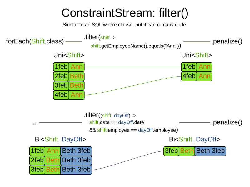
|
For performance reasons, using the join building block with the appropriate |
The following functions are required for filtering constraint streams of different cardinality:
Cardinality |
Filtering Predicate |
1 |
|
2 |
|
3 |
|
4 |
|
6.4.4. Joining
Joining is a way to increase stream cardinality and it is similar to the inner join
operation in SQL. As the following figure illustrates,
a join() creates a cartesian product of the streams being joined:
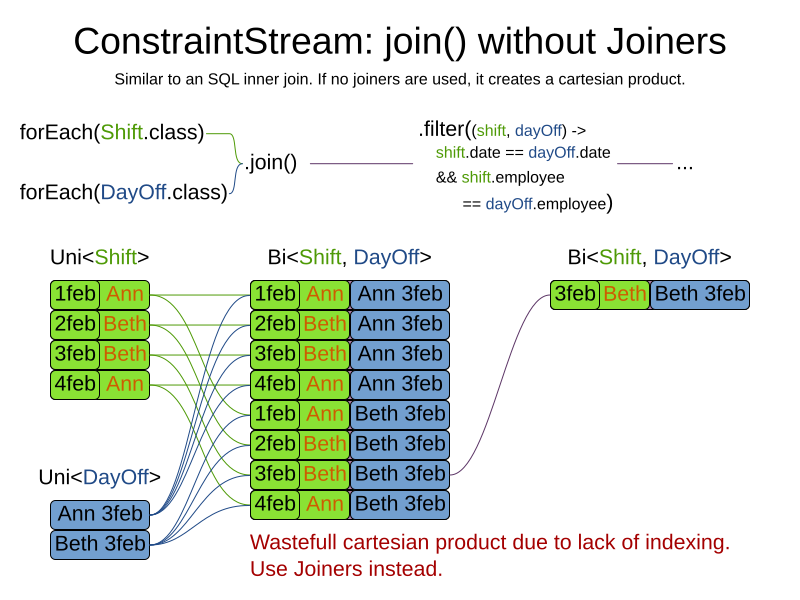
Doing this is inefficient if the resulting stream contains a lot of constraint matches that need to be filtered out immediately.
Instead, use a Joiner condition to restrict the joined matches only to those that are interesting:
For example:
import static org.optaplanner.core.api.score.stream.Joiners.*;
...
private Constraint shiftOnDayOff(ConstraintFactory constraintFactory) {
return constraintFactory.forEach(Shift.class)
.join(DayOff.class,
equal(Shift::getDate, DayOff::getDate),
equal(Shift::getEmployee, DayOff::getEmployee))
.penalize(HardSoftScore.ONE_HARD)
.asConstraint("Shift on an off-day");
}Through the Joiners class, the following Joiner conditions are supported to join two streams,
pairing a match from each side:
-
equal(): the paired matches have a property that areequals(). This relies onhashCode(). -
greaterThan(),greaterThanOrEqual(),lessThan()andlessThanOrEqual(): the paired matches have aComparableproperty following the prescribed ordering. -
overlapping(): the paired matches have two properties (a start and an end property) of the sameComparabletype that both represent an interval which overlap.
All Joiners methods have an overloaded method to use the same property of the same class on both stream sides.
For example, calling equal(Shift::getEmployee) is the same as calling equal(Shift::getEmployee, Shift::getEmployee).
|
If the other stream might match multiple times, but it must only impact the score once (for each element of the original stream), use ifExists instead. It does not create cartesian products and therefore generally performs better. |
6.4.5. Grouping and collectors
Grouping collects items in a stream according to user-provider criteria (also called "group key"), similar to what a
GROUP BY SQL clause does. Additionally, some grouping operations also accept one or more Collector instances, which
provide various aggregation functions. The following figure illustrates a simple groupBy() operation:
|
Objects used as group key must obey the general contract of For this reason, it is not recommended to use mutable objects (especially mutable collections) as group keys. If planning entities are used as group keys, their hashCode must not be computed off of planning variables. Failure to follow this recommendation may result in runtime exceptions being thrown. |
For example, the following code snippet first groups all processes by the computer they run on, sums up all the power
required by the processes on that computer using the ConstraintCollectors.sum(…) collector, and finally penalizes
every computer whose processes consume more power than is available.
import static org.optaplanner.core.api.score.stream.ConstraintCollectors.*;
...
private Constraint requiredCpuPowerTotal(ConstraintFactory constraintFactory) {
return constraintFactory.forEach(CloudProcess.class)
.groupBy(CloudProcess::getComputer, sum(CloudProcess::getRequiredCpuPower))
.filter((computer, requiredCpuPower) -> requiredCpuPower > computer.getCpuPower())
.penalize(HardSoftScore.ONE_HARD,
(computer, requiredCpuPower) -> requiredCpuPower - computer.getCpuPower())
.asConstraint("requiredCpuPowerTotal");
}|
Information might be lost during grouping.
In the previous example, |
There are several collectors available out of the box. You can also provide your own collectors by implementing the
org.optaplanner.core.api.score.stream.uni.UniConstraintCollector interface, or its Bi…, Tri… and Quad… counterparts.
6.4.5.1. Out-of-the-box collectors
The following collectors are provided out of the box:
6.4.5.1.1. count() collector
The ConstraintCollectors.count(…) counts all elements per group. For example, the following use of the collector
gives a number of items for two separate groups - one where the talks have unavailable speakers, and one where they
don’t.
private Constraint speakerAvailability(ConstraintFactory factory) {
return factory.forEach(Talk.class)
.groupBy(Talk::hasAnyUnavailableSpeaker, count())
.penalize(HardSoftScore.ONE_HARD,
(hasUnavailableSpeaker, count) -> ...)
.asConstraint("speakerAvailability");
}The count is collected in an int. Variants of this collector:
-
countLong()collects alongvalue instead of anintvalue.
To count a bi, tri or quad stream, use countBi(), countTri() or countQuad() respectively,
because - unlike the other built-in collectors - they aren’t overloaded methods due to Java’s generics erasure.
6.4.5.1.2. countDistinct() collector
The ConstraintCollectors.countDistinct(…) counts any element per group once, regardless of how many times it
occurs. For example, the following use of the collector gives a number of talks in each unique room.
private Constraint roomCount(ConstraintFactory factory) {
return factory.forEach(Talk.class)
.groupBy(Talk::getRoom, countDistinct())
.penalize(HardSoftScore.ONE_SOFT,
(room, count) -> ...)
.asConstraint("roomCount");
}The distinct count is collected in an int. Variants of this collector:
-
countDistinctLong()collects alongvalue instead of anintvalue.
6.4.5.1.3. sum() collector
To sum the values of a particular property of all elements per group, use the ConstraintCollectors.sum(…)
collector. The following code snippet first groups all processes by the computer they run on and sums up all the power
required by the processes on that computer using the ConstraintCollectors.sum(…) collector.
private Constraint requiredCpuPowerTotal(ConstraintFactory constraintFactory) {
return constraintFactory.forEach(CloudProcess.class)
.groupBy(CloudProcess::getComputer, sum(CloudProcess::getRequiredCpuPower))
.penalize(HardSoftScore.ONE_SOFT,
(computer, requiredCpuPower) -> requiredCpuPower)
.asConstraint("requiredCpuPowerTotal");
}The sum is collected in an int. Variants of this collector:
-
sumLong()collects alongvalue instead of anintvalue. -
sumBigDecimal()collects ajava.math.BigDecimalvalue instead of anintvalue. -
sumBigInteger()collects ajava.math.BigIntegervalue instead of anintvalue. -
sumDuration()collects ajava.time.Durationvalue instead of anintvalue. -
sumPeriod()collects ajava.time.Periodvalue instead of anintvalue. -
a generic
sum()variant for summing up custom types
6.4.5.1.4. average() collector
To calculate the average of a particular property of all elements per group, use the ConstraintCollectors.average(…)
collector.
The following code snippet first groups all processes by the computer they run on and averages all the power
required by the processes on that computer using the ConstraintCollectors.average(…) collector.
private Constraint requiredCpuPowerTotal(ConstraintFactory constraintFactory) {
return constraintFactory.forEach(CloudProcess.class)
.groupBy(CloudProcess::getComputer, average(CloudProcess::getRequiredCpuPower))
.penalize(HardSoftScore.ONE_SOFT,
(computer, averageCpuPower) -> averageCpuPower)
.asConstraint("averageCpuPower");
}The average is collected as a double, and the average of no elements is null.
Variants of this collector:
-
averageLong()collects alongvalue instead of anintvalue. -
averageBigDecimal()collects ajava.math.BigDecimalvalue instead of anintvalue, resulting in aBigDecimalaverage. -
averageBigInteger()collects ajava.math.BigIntegervalue instead of anintvalue, resulting in aBigDecimalaverage. -
averageDuration()collects ajava.time.Durationvalue instead of anintvalue, resulting in aDurationaverage.
6.4.5.1.5. min() and max() collectors
To extract the minimum or maximum per group, use the ConstraintCollectors.min(…) and
ConstraintCollectors.max(…) collectors respectively.
These collectors operate on values of properties which are Comparable (such as Integer, String or Duration),
although there are also variants of these collectors which allow you to provide your own Comparator.
The following example finds a computer which runs the most power-demanding process:
private Constraint computerWithBiggestProcess(ConstraintFactory constraintFactory) {
return constraintFactory.forEach(CloudProcess.class)
.groupBy(CloudProcess::getComputer, max(CloudProcess::getRequiredCpuPower))
.penalize(HardSoftScore.ONE_HARD,
(computer, biggestProcess) -> ...)
.asConstraint("computerWithBiggestProcess");
}|
|
6.4.5.1.6. toList(), toSet() and toMap() collectors
To extract all elements per group into a collection, use the ConstraintCollectors.toList(…).
The following example retrieves all processes running on a computer in a List:
private Constraint computerWithBiggestProcess(ConstraintFactory constraintFactory) {
return constraintFactory.forEach(CloudProcess.class)
.groupBy(CloudProcess::getComputer, toList())
.penalize(HardSoftScore.ONE_HARD,
(computer, processList) -> ...)
.asConstraint("computerAndItsProcesses");
}Variants of this collector:
-
toList()collects aListvalue. -
toSet()collects aSetvalue. -
toSortedSet()collects aSortedSetvalue. -
toMap()collects aMapvalue. -
toSortedMap()collects aSortedMapvalue.
|
The iteration order of elements in the resulting collection is not guaranteed to be stable,
unless it is a sorted collector such as |
6.4.5.2. Conditional collectors
The constraint collector framework enables you to create constraint collectors which will only collect in certain circumstances.
This is achieved using the ConstraintCollectors.conditionally(…) constraint collector.
This collector accepts a predicate, and another collector to which it will delegate if the predicate is true. The following example returns a count of long-running processes assigned to a given computer, excluding processes which are not long-running:
private Constraint computerWithLongRunningProcesses(ConstraintFactory constraintFactory) {
return constraintFactory.forEach(CloudProcess.class)
.groupBy(CloudProcess::getComputer, conditionally(
CloudProcess::isLongRunning,
count()
))
.penalize(HardSoftScore.ONE_HARD,
(computer, longRunningProcessCount) -> ...)
.asConstraint("longRunningProcesses");
}This is useful in situations where multiple collectors are used and only some of them need to be restricted.
If all of them needed to be restricted in the same way,
then applying a filter() before the grouping is preferable.
6.4.5.3. Composing collectors
The constraint collector framework enables you to create complex collectors utilizing simpler ones.
This is achieved using the ConstraintCollectors.compose(…) constraint collector.
This collector accepts 2 to 4 other constraint collectors,
and a function to merge their results into one.
The following example builds an average() constraint collector
using the count constraint collector and sum() constraint collector:
public static <A> UniConstraintCollector<A, ?, Double>
average(ToIntFunction<A> groupValueMapping) {
return compose(count(), sum(groupValueMapping), (count, sum) -> {
if (count == 0) {
return null;
} else {
return sum / (double) count;
}
});
}Similarly, the compose() collector enables you to work around the limitation of Constraint Stream cardinality
and use as many as 4 collectors in your groupBy() statements:
UniConstraintCollector<A, ?, Triple<Integer, Integer, Integer>> collector =
compose(count(),
min(),
max(),
(count, min, max) -> Triple.of(count, min, max));
}Such a composite collector returns a Triple instance which allows you to access
each of the sub collectors individually.
|
OptaPlanner does not provide any |
6.4.6. Conditional propagation
Conditional propagation enables you to exclude constraint matches from the constraint stream based on the presence or absence of some other object.
The following example penalizes computers which have at least one process running:
private Constraint runningComputer(ConstraintFactory constraintFactory) {
return constraintFactory.forEach(CloudComputer.class)
.ifExists(CloudProcess.class, Joiners.equal(Function.identity(), CloudProcess::getComputer))
.penalize(HardSoftScore.ONE_SOFT,
computer -> ...)
.asConstraint("runningComputer");
}Note the use of the ifExists() building block.
On UniConstraintStream, the ifExistsOther() building block is also available which is useful in situations where the
forEach() constraint match type is the same as the ifExists() type.
Conversely, if the ifNotExists() building block is used (as well as the ifNotExistsOther() building block on
UniConstraintStream) you can achieve the opposite effect:
private Constraint unusedComputer(ConstraintFactory constraintFactory) {
return constraintFactory.forEach(CloudComputer.class)
.ifNotExists(CloudProcess.class, Joiners.equal(Function.identity(), CloudProcess::getComputer))
.penalize(HardSoftScore.ONE_HARD,
computer -> ...)
.asConstraint("unusedComputer");
}Here, only the computers without processes running are penalized.
Also note the use of the Joiner class to limit the constraint matches.
For a description of available joiners, see joining.
Conditional propagation operates much like joining, with the exception of not increasing the
stream cardinality.
Matches from these building blocks are not available further down the stream.
|
For performance reasons, using conditional propagation with the appropriate |
6.4.7. Mapping tuples
Mapping enables you to transform each tuple in a constraint stream by applying a mapping function to it.
The result of such mapping is UniConstraintStream of the mapped tuples.
private Constraint computerWithBiggestProcess(ConstraintFactory constraintFactory) {
return constraintFactory.forEach(CloudProcess.class) // UniConstraintStream<CloudProcess>
.map(CloudProcess::getComputer) // UniConstraintStream<CloudComputer>
...
}|
In the example above, the mapping function produces duplicate tuples if two different |
6.4.7.1. Designing the mapping function
When designing the mapping function, follow these guidelines for optimal performance:
-
Keep the function pure. The mapping function should only depend on its input. That is, given the same input, it always returns the same output.
-
Keep the function bijective. No two input tuples should map to the same output tuple, or to tuples that are equal. Not following this recommendation creates a constraint stream with duplicate tuples, and may force you to use
distinct()later. -
Use immutable data carriers. The tuples returned by the mapping function should be immutable and identified by their contents and nothing else. If two tuples carry objects which equal one another, those two tuples should likewise equal and preferably be the same instance.
6.4.7.2. Dealing with duplicate tuples using distinct()
As a general rule, tuples in constraint streams are distinct. That is, no two tuples that equal one another. However, certain operations such as tuple mapping may produce constraint streams where that is not true.
If a constraint stream produces duplicate tuples, you can use the distinct() building block
to have the duplicate copies eliminated.
private Constraint computerWithBiggestProcess(ConstraintFactory constraintFactory) {
return constraintFactory.forEach(CloudProcess.class) // UniConstraintStream<CloudProcess>
.map(CloudProcess::getComputer) // UniConstraintStream<CloudComputer>
.distinct() // The same, each CloudComputer just once.
...
}|
There is a performance cost to |
6.4.8. Flattening
Flattening enables you to transform any Java Iterable (such as List or Set)
into a set of tuples, which are sent downstream.
(Similar to Java Stream’s flatMap(…).)
This is done by applying a mapping function to the final element in the source tuple.
private Constraint requiredJobRoles(ConstraintFactory constraintFactory) {
return constraintFactory.forEach(Person.class) // UniConstraintStream<Person>
.join(Job.class,
equal(Function.identity(), Job::getAssignee)) // BiConstraintStream<Person, Job>
.flattenLast(Job::getRequiredRoles) // BiConstraintStream<Person, Role>
.filter((person, requiredRole) -> ...)
...
}|
In the example above, the mapping function produces duplicate tuples
if |
6.5. Testing a constraint stream
Constraint streams include the Constraint Verifier unit testing harness.
To use it, first add a test scoped dependency to the optaplanner-test JAR.
6.5.1. Testing constraints in isolation
Consider the following constraint stream:
protected Constraint horizontalConflict(ConstraintFactory factory) {
return factory
.forEachUniquePair(Queen.class, equal(Queen::getRowIndex))
.penalize(SimpleScore.ONE)
.asConstraint("Horizontal conflict");
}The following example uses the Constraint Verifier API to create a simple unit test for the preceding constraint stream:
private ConstraintVerifier<NQueensConstraintProvider, NQueens> constraintVerifier
= ConstraintVerifier.build(new NQueensConstraintProvider(), NQueens.class, Queen.class);
@Test
public void horizontalConflictWithTwoQueens() {
Row row1 = new Row(0);
Column column1 = new Column(0);
Column column2 = new Column(1);
Queen queen1 = new Queen(0, row1, column1);
Queen queen2 = new Queen(1, row1, column2);
constraintVerifier.verifyThat(NQueensConstraintProvider::horizontalConflict)
.given(queen1, queen2)
.penalizesBy(1);
}This test ensures that the horizontal conflict constraint assigns a penalty of 1 when there are two queens on the same
row.
The following line creates a shared ConstraintVerifier instance and initializes the instance with the
NQueensConstraintProvider:
private ConstraintVerifier<NQueensConstraintProvider, NQueens> constraintVerifier
= ConstraintVerifier.build(new NQueensConstraintProvider(), NQueens.class, Queen.class);The @Test annotation indicates that the method is a unit test in a testing framework of your choice.
Constraint Verifier works with many testing frameworks including JUnit and AssertJ.
The first part of the test prepares the test data.
In this case, the test data includes two instances of the Queen planning entity and their dependencies
(Row, Column):
Row row1 = new Row(0);
Column column1 = new Column(0);
Column column2 = new Column(1);
Queen queen1 = new Queen(0, row1, column1);
Queen queen2 = new Queen(1, row1, column2);Further down, the following code tests the constraint:
constraintVerifier.verifyThat(NQueensConstraintProvider::horizontalConflict)
.given(queen1, queen2)
.penalizesBy(1);The verifyThat(…) call is used to specify a method on the NQueensConstraintProvider class which is under test.
This method must be visible to the test class, which the Java compiler enforces.
The given(…) call is used to enumerate all the facts that the constraint stream operates on.
In this case, the given(…) call takes the queen1 and queen2 instances previously created.
Alternatively, you can use a givenSolution(…) method here and provide a planning solution instead.
Finally, the penalizesBy(…) call completes the test, making sure that the horizontal conflict constraint, given
one Queen, results in a penalty of 1.
This number is a product of multiplying the match weight, as defined in the constraint stream, by the number of matches.
Alternatively, you can use a rewardsWith(…) call to check for rewards instead of penalties.
The method to use here depends on whether the constraint stream in question is terminated with a penalize or a
reward building block.
|
|
6.5.2. Testing all constraints together
In addition to testing individual constraints, you can test the entire ConstraintProvider instance.
Consider the following test:
@Test
public void givenFactsMultipleConstraints() {
Queen queen1 = new Queen(0, row1, column1);
Queen queen2 = new Queen(1, row2, column2);
Queen queen3 = new Queen(2, row3, column3);
constraintVerifier.verifyThat()
.given(queen1, queen2, queen3)
.scores(SimpleScore.of(-3));
}There are only two notable differences to the previous example.
First, the verifyThat() call takes no argument here, signifying that the entire ConstraintProvider instance is
being tested.
Second, instead of either a penalizesBy() or rewardsWith() call, the scores(…) method is used.
This runs the ConstraintProvider on the given facts and returns a sum of Scores of all constraint matches resulting
from the given facts.
Using this method, you ensure that the constraint provider does not miss any constraints and that the scoring function
remains consistent as your code base evolves.
It is therefore necessary for the given(…) method to list all planning entities and problem facts,
or provide the entire planning solution instead.
|
|
6.5.3. Testing in Quarkus
If you are using the optaplanner-quarkus extension, inject the ConstraintVerifier in your tests:
@QuarkusTest
public class MyConstraintProviderTest {
@Inject
ConstraintVerifier<MyConstraintProvider, MyPlanningSolution> constraintProvider;
}6.5.4. Testing in Spring Boot
If you are using the optaplanner-spring-boot-starter module, autowire the ConstraintVerifier in your tests:
@SpringBootTest
public class MyConstraintProviderTest {
@Autowired
ConstraintVerifier<MyConstraintProvider, MyPlanningSolution> constraintProvider;
}6.6. Variant implementation types
Constraint streams come in two flavors:
-
CS Drools (default): fast implementation that uses Drools underneath.
-
Bavet: even faster, more recent in-house implementation. To try it out set the
constraintStreamImplTypetoBAVETin your solver config:<solver xmlns="https://www.optaplanner.org/xsd/solver" xmlns:xsi="http://www.w3.org/2001/XMLSchema-instance" xsi:schemaLocation="https://www.optaplanner.org/xsd/solver https://www.optaplanner.org/xsd/solver/solver.xsd"> <scoreDirectorFactory> <constraintProviderClass>org.acme.schooltimetabling.solver.TimeTableConstraintProvider</constraintProviderClass> <!-- BAVET is experimental --> <constraintStreamImplType>BAVET</constraintStreamImplType> </scoreDirectorFactory> ... </solver>
Both of these variants implement the same ConstraintProvider API.
No Java code changes are necessary to switch between the two.
7. Drools score calculation (Deprecated)
|
Drools score calculation is deprecated and will be removed in a future major version of OptaPlanner. Consider switching to Constraint Streams with the help of our migration recipe. |
7.1. Overview
Implement your score calculation using the Drools rule engine. Every score constraint is written as one or more score rules.
-
Advantages:
-
Incremental score calculation for free
-
Because most DRL syntax uses forward chaining, it does incremental calculation without any extra code
-
-
Score constraints are isolated as separate rules
-
Easy to add or edit existing score rules
-
-
Flexibility to augment your score constraints by
-
Defining them in decision tables
-
Excel (XLS) spreadsheet
-
-
-
Performance optimizations in future versions for free
-
-
Disadvantages:
-
DRL learning curve
-
Usage of DRL
-
Polyglot fear can prohibit the use of a new language such as DRL in some organizations
-
-
|
Drools score calculation is not supported in Quarkus native mode. Consider switching to Constraint Streams. |
7.2. Drools score rules configuration
There are several ways to define where your score rules live.
7.2.1. A scoreDrl resource on the classpath
This is the easy way.
The score rules live in a DRL file which is provided as a classpath resource.
Just add the score rules DRL file in the solver configuration as a <scoreDrl> element:
<scoreDirectorFactory>
<scoreDrl>org/optaplanner/examples/nqueens/solver/nQueensConstraints.drl</scoreDrl>
</scoreDirectorFactory>In a typical project (following the Maven directory structure), that DRL file would be located at $PROJECT_DIR/src/main/resources/org/optaplanner/examples/nqueens/solver/nQueensConstraints.drl (even for a war project).
|
The |
Add multiple <scoreDrl> elements if the score rules are split across multiple DRL files.
Optionally, you can also set drools configuration properties:
<scoreDirectorFactory>
<scoreDrl>org/optaplanner/examples/nqueens/solver/nQueensConstraints.drl</scoreDrl>
<kieBaseConfigurationProperties>
<property name="drools.equalityBehavior" value="..." />
</kieBaseConfigurationProperties>
</scoreDirectorFactory>To enable property reactive by default, without a @propertyReactive on the domain classes,
add <drools.propertySpecific>ALWAYS</drools.propertySpecific> in there.
Otherwise OptaPlanner automatically changes the Drools default to ALLOWED so property reactive is not active by default.
7.2.2. A scoreDrlFile element
To use File on the local file system, instead of a classpath resource, add the score rules DRL file in the solver configuration as a <scoreDrlFile> element:
<scoreDirectorFactory>
<scoreDrlFile>/home/ge0ffrey/tmp/nQueensConstraints.drl</scoreDrlFile>
</scoreDirectorFactory>|
For portability reasons, a classpath resource is recommended over a File. An application built on one computer, but used on another computer, might not find the file on the same location. Worse, if they use a different Operating System, it is hard to choose a portable file path. |
Add multiple <scoreDrlFile> elements if the score rules are split across multiple DRL files.
7.3. Implementing a score rule
Here is an example of a score constraint implemented as a score rule in a DRL file:
rule "Horizontal conflict"
when
Queen($id : id, row != null, $i : rowIndex)
Queen(id > $id, rowIndex == $i)
then
scoreHolder.addConstraintMatch(kcontext, -1);
endThis score rule will fire once for every two queens with the same rowIndex.
The (id > $id) condition is needed to assure that for two queens A and B, it can only fire for (A, B) and not for (B, A), (A, A) or (B, B). Let us take a closer look at this score rule on this solution of four queens:
In this solution the Horizontal conflict score rule will fire for six queen couples: (A, B), (A, C), (A, D), (B, C), (B, D) and (C, D). Because none of the queens are on the same vertical or diagonal line, this solution will have a score of -6.
An optimal solution of four queens has a score of 0.
|
Notice that every score rule uses at least one planning entity class (directly or indirectly through a logically inserted fact). It is a waste of time to write a score rule that only relates to problem facts, as the consequence will never change during planning, no matter what the possible solution. |
A ScoreHolder instance is asserted into the KieSession as a global called scoreHolder.
The score rules need to (directly or indirectly) update that instance to influence the score of a solution state.
|
The |
7.4. Weighing score rules
If you’ve configured a constraint configuration, the score level and score weight of each constraint are beautifully decoupled from the constraint implementation, so they can be changed by the business users more easily.
In that case, use the reward() and penalize() methods of the ScoreHolder:
package org.optaplanner.examples.nqueens.solver;
...
global SimpleScoreHolder scoreHolder;
rule "Horizontal conflict"
when
Queen($id : id, row != null, $i : rowIndex)
Queen(id > $id, rowIndex == $i)
then
scoreHolder.penalize(kcontext);
end
// Vertical conflict is impossible due the model
rule "Ascending diagonal conflict"
when
Queen($id : id, row != null, $i : ascendingDiagonalIndex)
Queen(id > $id, ascendingDiagonalIndex == $i)
then
scoreHolder.penalize(kcontext);
end
rule "Descending diagonal conflict"
when
Queen($id : id, row != null, $i : descendingDiagonalIndex)
Queen(id > $id, descendingDiagonalIndex == $i)
then
scoreHolder.penalize(kcontext);
endThey automatically impact the score for each constraint match by the score weight defined in the constraint configuration.
The drl file must define a package (otherwise Drools defaults to defaultpkg)
and it must match with the constraint configuration's constraintPackage.
|
To learn more about the Drools rule language (DRL), consult the Drools documentation. |
The score weight of some constraints depends on the constraint match.
In these cases, provide a match weight to the reward() or penalize() methods.
The score impact is the constraint weight multiplied with the match weight.
For example in conference scheduling, the impact of a content conflict, depends on the number of shared content tags between 2 overlapping talks:
rule "Content conflict"
when
$talk1 : Talk(...)
$talk2 : Talk(...)
then
scoreHolder.penalize(kcontext,
$talk2.overlappingContentCount($talk1));
endPresume its constraint weight is set to 100soft.
So when 2 overlapping talks share only 1 content tag, the score is impacted by -100soft.
But when 2 overlapping talks share 3 content tags, the match weight is 3, so the score is impacted by -300soft.
If there is no constraint configuration, you’ll need to hard-code the weight in the constraint implementations:
global HardSoftScoreHolder scoreHolder;
// RoomCapacity: For each lecture, the number of students that attend the course must be less or equal
// than the number of seats of all the rooms that host its lectures.
rule "roomCapacity"
when
$room : Room($capacity : capacity)
$lecture : Lecture(room == $room, studentSize > $capacity, $studentSize : studentSize)
then
// Each student above the capacity counts as one point of penalty.
scoreHolder.addSoftConstraintMatch(kcontext, ($capacity - $studentSize));
end
// CurriculumCompactness: Lectures belonging to a curriculum should be adjacent
// to each other (i.e., in consecutive periods).
// For a given curriculum we account for a violation every time there is one lecture not adjacent
// to any other lecture within the same day.
rule "curriculumCompactness"
when
...
then
// Each isolated lecture in a curriculum counts as two points of penalty.
scoreHolder.addSoftConstraintMatch(kcontext, -2);
endNotice how addSoftConstraintMatch() specifies that it’s a soft constraint,
and needs a negative number to penalize each match. Otherwise it would reward such matches.
The parameter ($capacity - $studentSize) always results in a negative number because studentSize > $capacity.
7.5. Testing Drools-based constraints
Drools-based constraints come with a unit testing harness.
To use it, first add a test scoped dependency to the optaplanner-test jar to take advantage of the JUnit integration
and use the ScoreVerifier classes to test score rules in DRL (or a constraint match aware incremental score calculator).
For example, suppose you want to test these score rules:
global HardSoftScoreHolder scoreHolder;
rule "requiredCpuPowerTotal"
when
...
then
scoreHolder.addHardConstraintMatch(...);
end
...
rule "computerCost"
when
...
then
scoreHolder.addSoftConstraintMatch(...);
endFor each score rule, create a separate @Test that only tests the effect of that score rule on the score:
public class CloudBalancingScoreConstraintTest {
private HardSoftScoreVerifier<CloudBalance> scoreVerifier = new HardSoftScoreVerifier<>(
SolverFactory.createFromXmlResource(
"org/optaplanner/examples/cloudbalancing/solver/cloudBalancingSolverConfig.xml"));
@Test
public void requiredCpuPowerTotal() {
CloudComputer c1 = new CloudComputer(1L, 1000, 1, 1, 1);
CloudComputer c2 = new CloudComputer(2L, 200, 1, 1, 1);
CloudProcess p1 = new CloudProcess(1L, 700, 0, 0);
CloudProcess p2 = new CloudProcess(2L, 70, 0, 0);
CloudBalance solution = new CloudBalance(0L,
Arrays.asList(c1, c2),
Arrays.asList(p1, p2));
// Uninitialized
scoreVerifier.assertHardWeight("requiredCpuPowerTotal", 0, solution);
p1.setComputer(c1);
p2.setComputer(c1);
// Usage 700 + 70 is within capacity 1000 of c1
scoreVerifier.assertHardWeight("requiredCpuPowerTotal", 0, solution);
p1.setComputer(c2);
p2.setComputer(c2);
// Usage 700 + 70 is above capacity 200 of c2
scoreVerifier.assertHardWeight("requiredCpuPowerTotal", -570, solution);
}
...
@Test
public void computerCost() {
CloudComputer c1 = new CloudComputer(1L, 1, 1, 1, 200);
CloudComputer c2 = new CloudComputer(2L, 1, 1, 1, 30);
CloudProcess p1 = new CloudProcess(1L, 0, 0, 0);
CloudProcess p2 = new CloudProcess(2L, 0, 0, 0);
CloudBalance solution = new CloudBalance(0L,
Arrays.asList(c1, c2),
Arrays.asList(p1, p2));
// Uninitialized
scoreVerifier.assertSoftWeight("computerCost", 0, solution);
p1.setComputer(c1);
p2.setComputer(c1);
// Pay 200 for c1
scoreVerifier.assertSoftWeight("computerCost", -200, solution);
p2.setComputer(c2);
// Pay 200 + 30 for c1 and c2
scoreVerifier.assertSoftWeight("computerCost", -230, solution);
}
}There is a ScoreVerifier implementation for each Score implementation.
In the assertHardWeight() and assertSoftWeight() methods, the weight of the other score rules is ignored (even those of the same score level).
|
A ScoreVerifier does not work well to isolate score corruption,
use an |
8. Shadow variable
8.1. Introduction
A shadow variable is a planning variable whose correct value can be deduced from the state of the genuine planning variables. Even though such a variable violates the principle of normalization by definition, in some use cases it can be very practical to use a shadow variable, especially to express the constraints more naturally. For example in vehicle routing with time windows: the arrival time at a customer for a vehicle can be calculated based on the previously visited customers of that vehicle (and the known travel times between two locations).
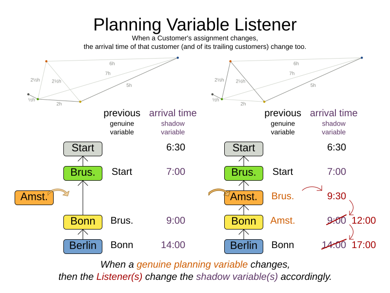
When the customers for a vehicle change, the arrival time for each customer is automatically adjusted. For more information, see the vehicle routing domain model.
From a score calculation perspective, a shadow variable is like any other planning variable. From an optimization perspective, OptaPlanner effectively only optimizes the genuine variables (and mostly ignores the shadow variables): it just assures that when a genuine variable changes, any dependent shadow variables are changed accordingly.
|
Any class that has at least one shadow variable, is a planning entity class (even if it has no genuine planning variables).
That class must be defined in the solver configuration and have a A genuine planning entity class has at least one genuine planning variable, but can have shadow variables too. A shadow planning entity class has no genuine planning variables and at least one shadow planning variable. |
There are several built-in shadow variables:
8.2. Bi-directional variable (inverse relation shadow variable)
Two variables are bi-directional if their instances always point to each other (unless one side points to null and the other side does not exist).
So if A references B, then B references A.
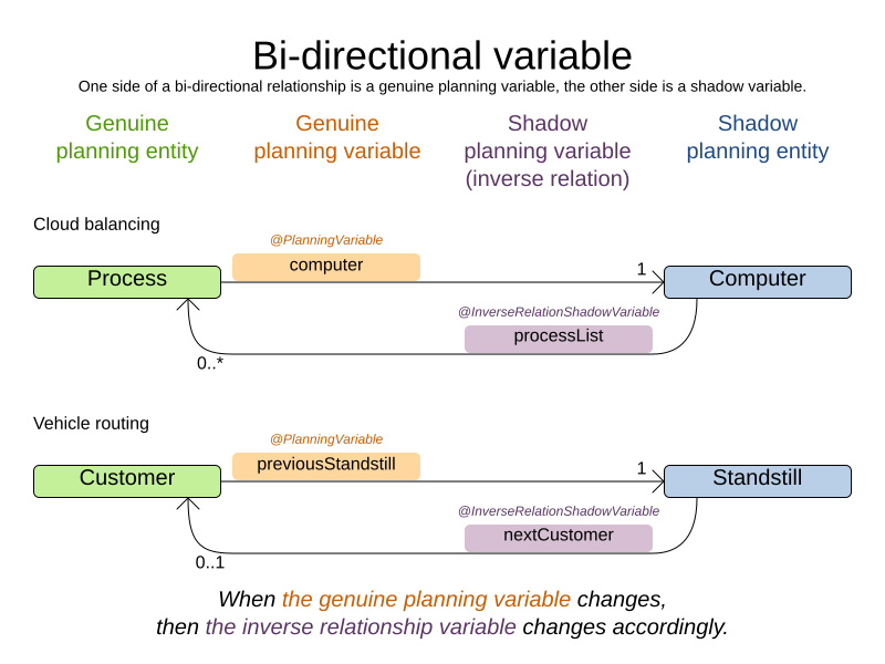
For a non-chained planning variable, the bi-directional relationship must be a many-to-one relationship. To map a bi-directional relationship between two planning variables, annotate the source side (which is the genuine side) as a normal planning variable:
@PlanningEntity
public class CloudProcess {
@PlanningVariable(...)
public CloudComputer getComputer() {
return computer;
}
public void setComputer(CloudComputer computer) {...}
}And then annotate the other side (which is the shadow side) with a @InverseRelationShadowVariable annotation on a Collection (usually a Set or List) property:
@PlanningEntity
public class CloudComputer {
@InverseRelationShadowVariable(sourceVariableName = "computer")
public List<CloudProcess> getProcessList() {
return processList;
}
}Register this class as a planning entity,
otherwise OptaPlanner won’t detect it and the shadow variable won’t update.
The sourceVariableName property is the name of the genuine planning variable on the return type of the getter
(so the name of the genuine planning variable on the other side).
|
The shadow property, which is |
For a chained planning variable, the bi-directional relationship is always a one-to-one relationship. In that case, the genuine side looks like this:
@PlanningEntity
public class Customer ... {
@PlanningVariable(graphType = PlanningVariableGraphType.CHAINED, ...)
public Standstill getPreviousStandstill() {
return previousStandstill;
}
public void setPreviousStandstill(Standstill previousStandstill) {...}
}And the shadow side looks like this:
@PlanningEntity
public class Standstill {
@InverseRelationShadowVariable(sourceVariableName = "previousStandstill")
public Customer getNextCustomer() {
return nextCustomer;
}
public void setNextCustomer(Customer nextCustomer) {...}
}Register this class as a planning entity, otherwise OptaPlanner won’t detect it and the shadow variable won’t update.
|
The input planning problem of a |
8.3. Anchor shadow variable
An anchor shadow variable is the anchor of a chained variable.
Annotate the anchor property as a @AnchorShadowVariable annotation:
@PlanningEntity
public class Customer {
@AnchorShadowVariable(sourceVariableName = "previousStandstill")
public Vehicle getVehicle() {...}
public void setVehicle(Vehicle vehicle) {...}
}This class should already be registered as a planning entity.
The sourceVariableName property is the name of the chained variable on the same entity class.
8.4. List variable shadow variables
When the planning entity uses a list variable, its elements can use a number of built-in shadow variables.
8.4.1. Inverse relation shadow variable
Use the same @InverseRelationShadowVariable annotation as with basic or chained planning variable to establish bi-directional relationship between the entity and the elements assigned to its list variable.
The type of the inverse shadow variable is the planning entity itself because there is a one-to-many relationship between the entity and the element classes.
The planning entity side has a genuine list variable:
@PlanningEntity
public class Vehicle {
@PlanningListVariable
public List<Customer> getCustomers() {
return customers;
}
public void setCustomers(List<Customer> customers) {...}
}On the element side:
-
Annotate the class with
@PlanningEntityto make it a shadow planning entity. -
Register this class as a planning entity, otherwise OptaPlanner won’t detect it and the shadow variable won’t update.
-
Create a property with the genuine planning entity type.
-
Annotate it with
@InverseRelationShadowVariableand setsourceVariableNameto the name of the genuine planning list variable.
@PlanningEntity
public class Customer {
@InverseRelationShadowVariable(sourceVariableName = "customers")
public Vehicle getVehicle() {
return vehicle;
}
public void setVehicle(Vehicle vehicle) {...}
}8.4.2. Previous and next element shadow variable
Use @PreviousElementShadowVariable or @NextElementShadowVariable to get a reference to an element that is assigned to the same entity’s list variable one index lower (previous element) or one index higher (next element).
|
The previous and next element shadow variables may be |
The planning entity side has a genuine list variable:
@PlanningEntity
public class Vehicle {
@PlanningListVariable
public List<Customer> getCustomers() {
return customers;
}
public void setCustomers(List<Customer> customers) {...}
}On the element side:
@PlanningEntity
public class Customer {
@PreviousElementShadowVariable(sourceVariableName = "customers")
public Customer getPreviousCustomer() {
return previousCustomer;
}
public void setPreviousCustomer(Customer previousCustomer) {...}
@NextElementShadowVariable(sourceVariableName = "customers")
public Customer getNextCustomer() {
return nextCustomer;
}
public void setNextCustomer(Customer nextCustomer) {...}8.5. Custom VariableListener
To update a shadow variable, OptaPlanner uses a VariableListener.
To define a custom shadow variable, write a custom VariableListener:
implement the interface and annotate it on the shadow variable that needs to change.
@PlanningVariable(...)
public Standstill getPreviousStandstill() {
return previousStandstill;
}
@ShadowVariable(
variableListenerClass = VehicleUpdatingVariableListener.class,
sourceVariableName = "previousStandstill")
public Vehicle getVehicle() {
return vehicle;
}Register this class as a planning entity if it isn’t already. Otherwise OptaPlanner won’t detect it and the shadow variable won’t update.
The sourceVariableName is the (genuine or shadow) variable that triggers changes to the annotated shadow variable.
If the source variable is declared on a different class than the annotated shadow variable’s class, also specify the sourceEntityClass and make sure the shadow variable’s class is registered as a planning entity.
Implement the VariableListener interface.
For example, the VehicleUpdatingVariableListener assures that every Customer in a chain has the same Vehicle, namely the chain’s anchor.
public class VehicleUpdatingVariableListener implements VariableListener<VehicleRoutingSolution, Customer> {
public void afterEntityAdded(ScoreDirector<VehicleRoutingSolution> scoreDirector, Customer customer) {
updateVehicle(scoreDirector, customer);
}
public void afterVariableChanged(ScoreDirector<VehicleRoutingSolution> scoreDirector, Customer customer) {
updateVehicle(scoreDirector, customer);
}
...
protected void updateVehicle(ScoreDirector<VehicleRoutingSolution> scoreDirector, Customer sourceCustomer) {
Standstill previousStandstill = sourceCustomer.getPreviousStandstill();
Vehicle vehicle = previousStandstill == null ? null : previousStandstill.getVehicle();
Customer shadowCustomer = sourceCustomer;
while (shadowCustomer != null && shadowCustomer.getVehicle() != vehicle) {
scoreDirector.beforeVariableChanged(shadowCustomer, "vehicle");
shadowCustomer.setVehicle(vehicle);
scoreDirector.afterVariableChanged(shadowCustomer, "vehicle");
shadowCustomer = shadowCustomer.getNextCustomer();
}
}
}|
A |
|
Any change of a shadow variable must be told to the |
8.5.1. Multiple source variables
If your custom variable listener needs multiple source variables to compute the shadow variable, annotate the shadow variable with multiple @ShadowVariable annotations, one per each source variable.
@PlanningVariable(...)
public ExecutionMode getExecutionMode() {
return executionMode;
}
@PlanningVariable(...)
public Integer getDelay() {
return delay;
}
@ShadowVariable(
variableListenerClass = PredecessorsDoneDateUpdatingVariableListener.class,
sourceVariableName = "executionMode")
@ShadowVariable(
variableListenerClass = PredecessorsDoneDateUpdatingVariableListener.class,
sourceVariableName = "delay")
public Integer getPredecessorsDoneDate() {
return predecessorsDoneDate;
}8.5.2. Piggyback shadow variable
If one VariableListener changes two or more shadow variables (because having two separate VariableListeners would be inefficient), then annotate only the first shadow variable with @ShadowVariable and specify the variableListenerClass there.
Use @PiggybackShadowVariable on each shadow variable updated by that variable listener and reference the first shadow variable:
@PlanningVariable(...)
public Standstill getPreviousStandstill() {
return previousStandstill;
}
@ShadowVariable(
variableListenerClass = TransportTimeAndCapacityUpdatingVariableListener.class,
sourceVariableName = "previousStandstill")
public Integer getTransportTime() {
return transportTime;
}
@PiggybackShadowVariable(shadowVariableName = "transportTime")
public Integer getCapacity() {
return capacity;
}8.5.3. Shadow variable cloning
A shadow variable’s value (just like a genuine variable’s value)
isn’t planning cloned by the default solution cloner,
unless it can easily prove that it must be planning cloned (for example the property type is a planning entity class).
Specifically shadow variables of type List, Set, Collection or Map usually need to be planning cloned
to avoid corrupting the best solution when the working solution changes.
To planning clone a shadow variable, add @DeepPlanningClone annotation:
@DeepPlanningClone
@ShadowVariable(...)
private Map<LocalDateTime, Integer> usedManHoursPerDayMap;8.6. VariableListener triggering order
All shadow variables are triggered by a VariableListener, regardless if it’s a built-in or a custom shadow variable.
The genuine and shadow variables form a graph, that determines the order in which the afterEntityAdded(), afterVariableChanged() and afterEntityRemoved() methods are called:
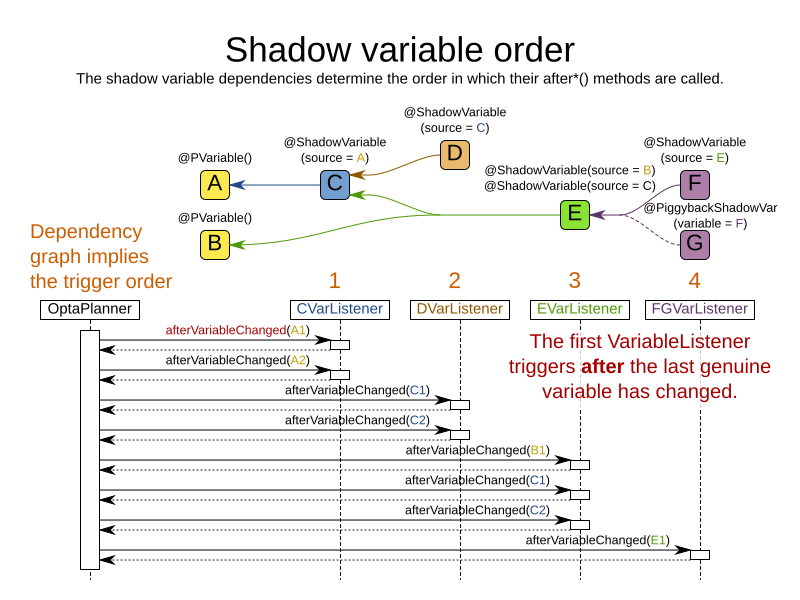
|
In the example above, D could have also been ordered after E (or F) because there is no direct or indirect dependency between D and E (or F). |
OptaPlanner guarantees that:
-
The first
VariableListener'safter*()methods trigger after the last genuine variable has changed. Therefore the genuine variables (A and B in the example above) are guaranteed to be in a consistent state across all its instances (with values A1, A2 and B1 in the example above) because the entireMovehas been applied. -
The second
VariableListener'safter*()methods trigger after the last first shadow variable has changed. Therefore the first shadow variable (C in the example above) are guaranteed to be in a consistent state across all its instances (with values C1 and C2 in the example above). And of course the genuine variables too. -
And so forth.
OptaPlanner does not guarantee the order in which the after*() methods are called for the sameVariableListener with different parameters (such as A1 and A2 in the example above), although they are likely to be in the order in which they were affected.
By default, OptaPlanner does not guarantee that the events are unique.
For example, if a shadow variable on an entity is changed twice in the same move (for example by two different genuine variables), then that will cause the same event twice on the VariableListeners that are listening to that original shadow variable.
To avoid dealing with that complexity, overwrite the method requiresUniqueEntityEvents() to receive unique events at the cost of a small performance penalty:
public class StartTimeUpdatingVariableListener implements VariableListener<TaskAssigningSolution, Task> {
@Override
public boolean requiresUniqueEntityEvents() {
return true;
}
...
}9. Optimization algorithms
9.1. Search space size in the real world
The number of possible solutions for a planning problem can be mind blowing. For example:
-
Four queens has
256possible solutions (4^4) and two optimal solutions. -
Five queens has
3125possible solutions (5^5) and one optimal solution. -
Eight queens has
16777216possible solutions (8^8) and 92 optimal solutions. -
64 queens has more than
10^115possible solutions (64^64). -
Most real-life planning problems have an incredible number of possible solutions and only one or a few optimal solutions.
For comparison: the minimal number of atoms in the known universe (10^80). As a planning problem gets bigger, the search space tends to blow up really fast. Adding only one extra planning entity or planning value can heavily multiply the running time of some algorithms.
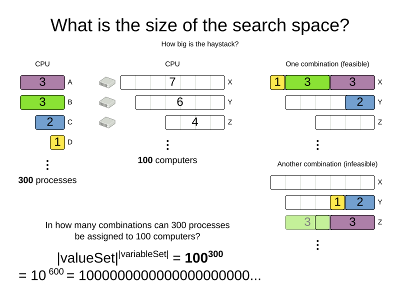
Calculating the number of possible solutions depends on the design of the domain model:
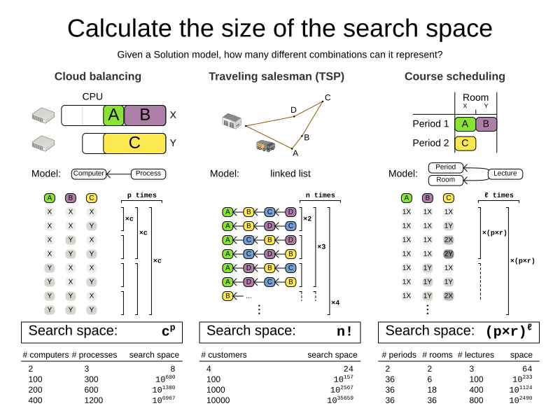
|
This search space size calculation includes infeasible solutions (if they can be represented by the model), because:
Even in cases where adding some of the hard constraints in the formula is practical (for example, Course Scheduling), the resulting search space is still huge. |
An algorithm that checks every possible solution (even with pruning, such as in Branch And Bound) can easily run for billions of years on a single real-life planning problem. The aim is to find the best solution in the available timeframe. Planning competitions (such as the International Timetabling Competition) show that Local Search variations (Tabu Search, Simulated Annealing, Late Acceptance, …) usually perform best for real-world problems given real-world time limitations.
9.2. Does OptaPlanner find the optimal solution?
The business wants the optimal solution, but they also have other requirements:
-
Scale out: Large production data sets must not crash and have also good results.
-
Optimize the right problem: The constraints must match the actual business needs.
-
Available time: The solution must be found in time, before it becomes useless to execute.
-
Reliability: Every data set must have at least a decent result (better than a human planner).
Given these requirements, and despite the promises of some salesmen, it is usually impossible for anyone or anything to find the optimal solution. Therefore, OptaPlanner focuses on finding the best solution in available time. In "realistic, independent competitions", it often comes out as the best reusable software.
The nature of NP-complete problems make scaling a prime concern.
|
The quality of a result from a small data set is no indication of the quality of a result from a large data set. |
Scaling issues cannot be mitigated by hardware purchases later on. Start testing with a production sized data set as soon as possible. Do not assess quality on small data sets (unless production encounters only such data sets). Instead, solve a production sized data set and compare the results of longer executions, different algorithms and - if available - the human planner.
9.3. Architecture overview
OptaPlanner is the first framework to combine optimization algorithms (metaheuristics, …) with score calculation by a rule engine (such as Drools). This combination is very efficient, because:
-
A rule engine, such as Drools, is great for calculating the score of a solution of a planning problem. It makes it easy and scalable to add additional soft or hard constraints. It does incremental score calculation (deltas) without any extra code. However it tends to be not suitable to actually find new solutions.
-
An optimization algorithm is great at finding new improving solutions for a planning problem, without necessarily brute-forcing every possibility. However, it needs to know the score of a solution and offers no support in calculating that score efficiently.
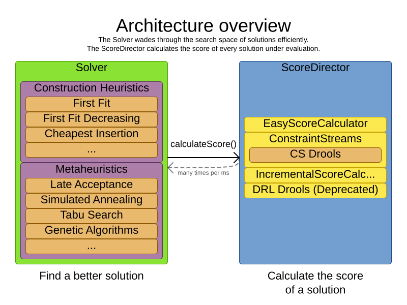
9.4. Optimization algorithms overview
OptaPlanner supports three families of optimization algorithms: Exhaustive Search, Construction Heuristics and Metaheuristics. In practice, Metaheuristics (in combination with Construction Heuristics to initialize) are the recommended choice:
Each of these algorithm families have multiple optimization algorithms:
| Algorithm | Scalable? | Optimal? | Easy to use? | Tweakable? | Requires CH? |
|---|---|---|---|---|---|
Exhaustive Search (ES) |
|||||
0/5 |
5/5 |
5/5 |
0/5 |
No |
|
0/5 |
5/5 |
4/5 |
2/5 |
No |
|
Construction heuristics (CH) |
|||||
5/5 |
1/5 |
5/5 |
1/5 |
No |
|
5/5 |
2/5 |
4/5 |
2/5 |
No |
|
5/5 |
2/5 |
4/5 |
2/5 |
No |
|
5/5 |
2/5 |
4/5 |
2/5 |
No |
|
5/5 |
2/5 |
4/5 |
2/5 |
No |
|
5/5 |
2/5 |
4/5 |
2/5 |
No |
|
3/5 |
2/5 |
5/5 |
2/5 |
No |
|
3/5 |
2/5 |
5/5 |
2/5 |
No |
|
Metaheuristics (MH) |
|||||
Local Search (LS) |
|||||
5/5 |
2/5 |
4/5 |
3/5 |
Yes |
|
5/5 |
4/5 |
3/5 |
5/5 |
Yes |
|
5/5 |
4/5 |
2/5 |
5/5 |
Yes |
|
5/5 |
4/5 |
3/5 |
5/5 |
Yes |
|
5/5 |
4/5 |
3/5 |
5/5 |
Yes |
|
5/5 |
4/5 |
3/5 |
5/5 |
Yes |
|
3/5 |
3/5 |
2/5 |
5/5 |
Yes |
|
Evolutionary Algorithms (EA) |
|||||
3/5 |
3/5 |
2/5 |
5/5 |
Yes |
|
3/5 |
3/5 |
2/5 |
5/5 |
Yes |
|
To learn more about metaheuristics, see Essentials of Metaheuristics or Clever Algorithms.
9.5. Which optimization algorithms should I use?
The best optimization algorithms configuration to use depends heavily on your use case. However, this basic procedure provides a good starting configuration that will produce better than average results.
-
Start with a quick configuration that involves little or no configuration and optimization code: See First Fit.
-
Next, implement planning entity difficulty comparison and turn it into First Fit Decreasing.
-
Next, add Late Acceptance behind it:
-
First Fit Decreasing.
-
At this point, the return on invested time lowers and the result is likely to be sufficient.
However, this can be improved at a lower return on invested time. Use the Benchmarker and try a couple of different Tabu Search, Simulated Annealing and Late Acceptance configurations, for example:
-
First Fit Decreasing: Tabu Search.
Use the Benchmarker to improve the values for the size parameters.
Other experiments can also be run. For example, the following multiple algorithms can be combined together:
-
First Fit Decreasing
-
Late Acceptance (relatively long time)
-
Tabu Search (relatively short time)
9.6. Power tweaking or default parameter values
Many optimization algorithms have parameters that affect results and scalability. OptaPlanner applies configuration by exception, so all optimization algorithms have default parameter values. This is very similar to the Garbage Collection parameters in a JVM: most users have no need to tweak them, but power users often do.
The default parameter values are sufficient for many cases (and especially for prototypes), but if development time allows, it may be beneficial to power tweak them with the benchmarker for better results and scalability on a specific use case. The documentation for each optimization algorithm also declares the advanced configuration for power tweaking.
|
The default value of parameters will change between minor versions, to improve them for most users. The advanced configuration can be used to prevent unwanted changes, however, this is not recommended. |
9.7. Solver phase
A Solver can use multiple optimization algorithms in sequence.
Each optimization algorithm is represented by one solver Phase.
There is never more than one Phase solving at the same time.
|
Some |
Here is a configuration that runs three phases in sequence:
<solver xmlns="https://www.optaplanner.org/xsd/solver" xmlns:xsi="http://www.w3.org/2001/XMLSchema-instance"
xsi:schemaLocation="https://www.optaplanner.org/xsd/solver https://www.optaplanner.org/xsd/solver/solver.xsd">
...
<constructionHeuristic>
... <!-- First phase: First Fit Decreasing -->
</constructionHeuristic>
<localSearch>
... <!-- Second phase: Late Acceptance -->
</localSearch>
<localSearch>
... <!-- Third phase: Tabu Search -->
</localSearch>
</solver>The solver phases are run in the order defined by solver configuration.
-
When the first
Phaseterminates, the secondPhasestarts, and so on. -
When the last
Phaseterminates, theSolverterminates.
Usually, a Solver will first run a construction heuristic and then run one or multiple metaheuristics:
If no phases are configured, OptaPlanner will default to a Construction Heuristic phase followed by a Local Search phase.
Some phases (especially construction heuristics) will terminate automatically.
Other phases (especially metaheuristics) will only terminate if the Phase is configured to terminate:
<solver xmlns="https://www.optaplanner.org/xsd/solver" xmlns:xsi="http://www.w3.org/2001/XMLSchema-instance"
xsi:schemaLocation="https://www.optaplanner.org/xsd/solver https://www.optaplanner.org/xsd/solver/solver.xsd">
...
<termination><!-- Solver termination -->
<secondsSpentLimit>90</secondsSpentLimit>
</termination>
<localSearch>
<termination><!-- Phase termination -->
<secondsSpentLimit>60</secondsSpentLimit><!-- Give the next phase a chance to run too, before the Solver terminates -->
</termination>
...
</localSearch>
<localSearch>
...
</localSearch>
</solver>If the Solver terminates (before the last Phase terminates itself),
the current phase is terminated and all subsequent phases will not run.
9.8. Scope overview
A solver will iteratively run phases. Each phase will usually iteratively run steps. Each step, in turn, usually iteratively runs moves. These form four nested scopes:
-
Solver
-
Phase
-
Step
-
Move
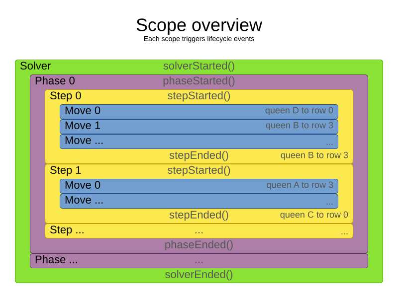
Configure logging to display the log messages of each scope.
9.9. Termination
Not all phases terminate automatically and may take a significant amount of time.
A Solver can be terminated synchronously by up-front configuration, or asynchronously from another thread.
Metaheuristic phases in particular need to be instructed to stop solving. This can be because of a number of reasons, for example, if the time is up, or the perfect score has been reached just before its solution is used. Finding the optimal solution cannot be relied on (unless you know the optimal score), because a metaheuristic algorithm is generally unaware of the optimal solution.
This is not an issue for real-life problems, as finding the optimal solution may take more time than is available. Finding the best solution in the available time is the most important outcome.
|
If no termination is configured (and a metaheuristic algorithm is used), the |
For synchronous termination, configure a Termination on a Solver or a Phase when it needs to stop.
The built-in implementations of these should be sufficient,
but custom terminations are supported too.
Every Termination can calculate a time gradient (needed for some optimization algorithms),
which is a ratio between the time already spent solving and the estimated entire solving time of the Solver or Phase.
9.9.1. Time spent termination
Terminates when an amount of time has been used.
<termination>
<!-- 2 minutes and 30 seconds in ISO 8601 format P[n]Y[n]M[n]DT[n]H[n]M[n]S -->
<spentLimit>PT2M30S</spentLimit>
</termination>Alternatively to a java.util.Duration in ISO 8601 format, you can also use:
-
Milliseconds
<termination> <millisecondsSpentLimit>500</millisecondsSpentLimit> </termination> -
Seconds
<termination> <secondsSpentLimit>10</secondsSpentLimit> </termination> -
Minutes
<termination> <minutesSpentLimit>5</minutesSpentLimit> </termination> -
Hours
<termination> <hoursSpentLimit>1</hoursSpentLimit> </termination> -
Days
<termination> <daysSpentLimit>2</daysSpentLimit> </termination>
Multiple time types can be used together, for example to configure 150 minutes, either configure it directly:
<termination>
<minutesSpentLimit>150</minutesSpentLimit>
</termination>Or use a combination that sums up to 150 minutes:
<termination>
<hoursSpentLimit>2</hoursSpentLimit>
<minutesSpentLimit>30</minutesSpentLimit>
</termination>|
This
|
9.9.2. Unimproved time spent termination
Terminates when the best score has not improved in a specified amount of time. Each time a new best solution is found, the timer basically resets.
<localSearch>
<termination>
<!-- 2 minutes and 30 seconds in ISO 8601 format P[n]Y[n]M[n]DT[n]H[n]M[n]S -->
<unimprovedSpentLimit>PT2M30S</unimprovedSpentLimit>
</termination>
</localSearch>Alternatively to a java.util.Duration in ISO 8601 format, you can also use:
-
Milliseconds
<localSearch> <termination> <unimprovedMillisecondsSpentLimit>500</unimprovedMillisecondsSpentLimit> </termination> </localSearch> -
Seconds
<localSearch> <termination> <unimprovedSecondsSpentLimit>10</unimprovedSecondsSpentLimit> </termination> </localSearch> -
Minutes
<localSearch> <termination> <unimprovedMinutesSpentLimit>5</unimprovedMinutesSpentLimit> </termination> </localSearch> -
Hours
<localSearch> <termination> <unimprovedHoursSpentLimit>1</unimprovedHoursSpentLimit> </termination> </localSearch> -
Days
<localSearch> <termination> <unimprovedDaysSpentLimit>1</unimprovedDaysSpentLimit> </termination> </localSearch>
Just like time spent termination, combinations are summed up.
It is preffered to configure this termination on a specific Phase (such as <localSearch>) instead of on the Solver itself.
|
This
|
Optionally, configure a score difference threshold by which the best score must improve in the specified time.
For example, if the score doesn’t improve by at least 100 soft points every 30 seconds or less, it terminates:
<localSearch>
<termination>
<unimprovedSecondsSpentLimit>30</unimprovedSecondsSpentLimit>
<unimprovedScoreDifferenceThreshold>0hard/100soft</unimprovedScoreDifferenceThreshold>
</termination>
</localSearch>If the score improves by 1 hard point and drops 900 soft points, it’s still meets the threshold,
because 1hard/-900soft is larger than the threshold 0hard/100soft.
On the other hand, a threshold of 1hard/0soft is not met by any new best solution
that improves 1 hard point at the expense of 1 or more soft points,
because 1hard/-100soft is smaller than the threshold 1hard/0soft.
To require a feasibility improvement every 30 seconds while avoiding the pitfall above,
use a wildcard * for lower score levels that are allowed to deteriorate if a higher score level improves:
<localSearch>
<termination>
<unimprovedSecondsSpentLimit>30</unimprovedSecondsSpentLimit>
<unimprovedScoreDifferenceThreshold>1hard/*soft</unimprovedScoreDifferenceThreshold>
</termination>
</localSearch>This effectively implies a threshold of 1hard/-2147483648soft, because it relies on Integer.MIN_VALUE.
9.9.3. BestScoreTermination
BestScoreTermination terminates when a certain score has been reached.
Use this Termination where the perfect score is known, for example for four queens (which uses a SimpleScore):
<termination>
<bestScoreLimit>0</bestScoreLimit>
</termination>A planning problem with a HardSoftScore may look like this:
<termination>
<bestScoreLimit>0hard/-5000soft</bestScoreLimit>
</termination>A planning problem with a BendableScore with three hard levels and one soft level may look like this:
<termination>
<bestScoreLimit>[0/0/0]hard/[-5000]soft</bestScoreLimit>
</termination>In this instance, Termination once a feasible solution has been reached is not practical because it requires a bestScoreLimit such as 0hard/-2147483648soft. Use the next termination instead.
9.9.4. BestScoreFeasibleTermination
Terminates as soon as a feasible solution has been discovered.
<termination>
<bestScoreFeasible>true</bestScoreFeasible>
</termination>This Termination is usually combined with other terminations.
9.9.5. StepCountTermination
Terminates when a number of steps has been reached. This is useful for hardware performance independent runs.
<localSearch>
<termination>
<stepCountLimit>100</stepCountLimit>
</termination>
</localSearch>This Termination can only be used for a Phase (such as <localSearch>), not for the Solver itself.
9.9.6. UnimprovedStepCountTermination
Terminates when the best score has not improved in a number of steps. This is useful for hardware performance independent runs.
<localSearch>
<termination>
<unimprovedStepCountLimit>100</unimprovedStepCountLimit>
</termination>
</localSearch>If the score has not improved recently, it is unlikely to improve in a reasonable timeframe. It has been observed that once a new best solution is found (even after a long time without improvement on the best solution), the next few steps tend to improve the best solution.
This Termination can only be used for a Phase (such as <localSearch>), not for the Solver itself.
9.9.7. ScoreCalculationCountTermination
ScoreCalculationCountTermination terminates when a number of score calculations have been reached.
This is often the sum of the number of moves and the number of steps.
This is useful for benchmarking.
<termination>
<scoreCalculationCountLimit>100000</scoreCalculationCountLimit>
</termination>Switching EnvironmentMode can heavily impact when this termination ends.
9.9.8. Combining multiple terminations
Terminations can be combined, for example: terminate after 100 steps or if a score of 0 has been reached:
<termination>
<terminationCompositionStyle>OR</terminationCompositionStyle>
<bestScoreLimit>0</bestScoreLimit>
<stepCountLimit>100</stepCountLimit>
</termination>Alternatively you can use AND, for example: terminate after reaching a feasible score of at least -100 and no improvements in 5 steps:
<termination>
<terminationCompositionStyle>AND</terminationCompositionStyle>
<bestScoreLimit>-100</bestScoreLimit>
<unimprovedStepCountLimit>5</unimprovedStepCountLimit>
</termination>This example ensures it does not just terminate after finding a feasible solution, but also completes any obvious improvements on that solution before terminating.
9.9.9. Asynchronous termination from another thread
Asynchronous termination cannot be configured by a Termination as it is impossible to predict when and if it will occur.
For example, a user action or a server restart could require a solver to terminate earlier than predicted.
To terminate a solver from another thread asynchronously
call the terminateEarly() method from another thread:
solver.terminateEarly();The solver then terminates at its earliest convenience.
After termination, the Solver.solve(Solution) method returns in the solver thread (which is the original thread that called it).
|
When an To guarantee a graceful shutdown of a thread pool that contains solver threads,
an interrupt of a solver thread has the same effect as calling |
9.10. SolverEventListener
Each time a new best solution is found, a new BestSolutionChangedEvent is fired in the Solver thread.
To listen to such events, add a SolverEventListener to the Solver:
public interface Solver<Solution_> {
...
void addEventListener(SolverEventListener<S> eventListener);
void removeEventListener(SolverEventListener<S> eventListener);
}The BestSolutionChangedEvent's newBestSolution may not be initialized or feasible.
Use the isFeasible() method on BestSolutionChangedEvent's new best Score to detect such cases:
solver.addEventListener(new SolverEventListener<CloudBalance>() {
public void bestSolutionChanged(BestSolutionChangedEvent<CloudBalance> event) {
// Ignore infeasible (including uninitialized) solutions
if (event.getNewBestSolution().getScore().isFeasible()) {
...
}
}
});Use Score.isSolutionInitialized() instead of Score.isFeasible() to only ignore uninitialized solutions, but also accept infeasible solutions.
|
The |
9.11. Custom solver phase
Run a custom optimization algorithm between phases or before the first phase to initialize the solution, or to get a better score quickly.
You will still want to reuse the score calculation.
For example, to implement a custom Construction Heuristic without implementing an entire Phase.
|
Most of the time, a custom solver phase is not worth the development time investment.
The supported Constructions Heuristics are configurable (use the Benchmarker to tweak them),
|
The CustomPhaseCommand interface appears as follows:
public interface CustomPhaseCommand<Solution_> {
...
void changeWorkingSolution(ScoreDirector<Solution_> scoreDirector);
}For example, implement CustomPhaseCommand and its changeWorkingSolution() method:
public class ToOriginalMachineSolutionInitializer extends AbstractCustomPhaseCommand<MachineReassignment> {
public void changeWorkingSolution(ScoreDirector<MachineReassignment> scoreDirector) {
MachineReassignment machineReassignment = scoreDirector.getWorkingSolution();
for (MrProcessAssignment processAssignment : machineReassignment.getProcessAssignmentList()) {
scoreDirector.beforeVariableChanged(processAssignment, "machine");
processAssignment.setMachine(processAssignment.getOriginalMachine());
scoreDirector.afterVariableChanged(processAssignment, "machine");
scoreDirector.triggerVariableListeners();
}
}
}|
Any change on the planning entities in a |
|
Do not change any of the problem facts in a |
Configure the CustomPhaseCommand in the solver configuration:
<solver xmlns="https://www.optaplanner.org/xsd/solver" xmlns:xsi="http://www.w3.org/2001/XMLSchema-instance"
xsi:schemaLocation="https://www.optaplanner.org/xsd/solver https://www.optaplanner.org/xsd/solver/solver.xsd">
...
<customPhase>
<customPhaseCommandClass>org.optaplanner.examples.machinereassignment.solver.solution.initializer.ToOriginalMachineSolutionInitializer</customPhaseCommandClass>
</customPhase>
... <!-- Other phases -->
</solver>Configure multiple customPhaseCommandClass instances to run them in sequence.
|
If the changes of a |
|
If the |
To configure values of a CustomPhaseCommand dynamically in the solver configuration
(so the Benchmarker can tweak those parameters),
add the customProperties element and use custom properties:
<customPhase>
<customPhaseCommandClass>...MyCustomPhase</customPhaseCommandClass>
<customProperties>
<property name="mySelectionSize" value="5"/>
</customProperties>
</customPhase>9.12. No change solver phase
In rare cases, it’s useful not to run any solver phases.
But by default, configuring no phase will trigger running the default phases.
To avoid those, configure a NoChangePhase:
<solver xmlns="https://www.optaplanner.org/xsd/solver" xmlns:xsi="http://www.w3.org/2001/XMLSchema-instance"
xsi:schemaLocation="https://www.optaplanner.org/xsd/solver https://www.optaplanner.org/xsd/solver/solver.xsd">
...
<noChangePhase/>
</solver>9.13. Multithreaded solving
There are several ways of doing multithreaded solving:
-
Multitenancy: solve different datasets in parallel
-
The
SolverManagerwill make it even easier to set this up, in a future version.
-
-
Multi bet solving: solve 1 dataset with multiple, isolated solvers and take the best result.
-
Not recommended: This is a marginal gain for a high cost of hardware resources.
-
Use the Benchmarker during development to determine the most appropriate algorithm, although that’s only on average.
-
Use multithreaded incremental solving instead.
-
-
Partitioned Search: Split 1 dataset in multiple parts and solve them independently.
-
Configure a Partitioned Search.
-
-
Multithreaded incremental solving: solve 1 dataset with multiple threads without sacrificing incremental score calculation.
-
Donate a portion of your CPU cores to OptaPlanner to scale up the score calculation speed and get the same results in fraction of the time.
-
Configure multithreaded incremental solving.
-
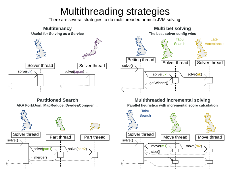
|
A logging level of |
9.13.1. @PlanningId
For some functionality (such as multithreaded solving and real-time planning), OptaPlanner needs to map problem facts and planning entities to an ID. OptaPlanner uses that ID to rebase a move from one thread’s solution state to another’s.
To enable such functionality, specify the @PlanningId annotation on the identification field or getter method,
for example on the database ID:
public class CloudComputer {
@PlanningId
private Long id;
...
}Or alternatively, on another type of ID:
public class User {
@PlanningId
private String username;
...
}A @PlanningId property must be:
-
Unique for that specific class
-
It does not need to be unique across different problem fact classes (unless in that rare case that those classes are mixed in the same value range or planning entity collection).
-
-
An instance of a type that implements
Object.hashCode()andObject.equals().-
It’s recommended to use the type
Integer,int,Long,long,StringorUUID.
-
-
Never
nullby the timeSolver.solve()is called.
9.13.2. Custom thread factory (WildFly, Android, GAE, …)
The threadFactoryClass allows to plug in a custom ThreadFactory for environments
where arbitrary thread creation should be avoided,
such as most application servers (including WildFly), Android, or Google App Engine.
Configure the ThreadFactory on the solver to create the move threads
and the Partition Search threads with it:
<solver xmlns="https://www.optaplanner.org/xsd/solver" xmlns:xsi="http://www.w3.org/2001/XMLSchema-instance"
xsi:schemaLocation="https://www.optaplanner.org/xsd/solver https://www.optaplanner.org/xsd/solver/solver.xsd">
<threadFactoryClass>...MyAppServerThreadFactory</threadFactoryClass>
...
</solver>9.13.3. Multithreaded incremental solving
Enable multithreaded incremental solving by adding a @PlanningId annotation
on every planning entity class and planning value class.
Then configure a moveThreadCount:
<solver xmlns="https://www.optaplanner.org/xsd/solver" xmlns:xsi="http://www.w3.org/2001/XMLSchema-instance"
xsi:schemaLocation="https://www.optaplanner.org/xsd/solver https://www.optaplanner.org/xsd/solver/solver.xsd">
<moveThreadCount>AUTO</moveThreadCount>
...
</solver>That one extra line heavily improves the score calculation speed, presuming that your machine has enough free CPU cores.
Advanced configuration:
<solver xmlns="https://www.optaplanner.org/xsd/solver" xmlns:xsi="http://www.w3.org/2001/XMLSchema-instance"
xsi:schemaLocation="https://www.optaplanner.org/xsd/solver https://www.optaplanner.org/xsd/solver/solver.xsd">
<moveThreadCount>4</moveThreadCount>
<moveThreadBufferSize>10</moveThreadBufferSize>
<threadFactoryClass>...MyAppServerThreadFactory</threadFactoryClass>
...
</solver>A moveThreadCount of 4 saturates almost 5 CPU cores:
the 4 move threads fill up 4 CPU cores completely
and the solver thread uses most of another CPU core.
The following moveThreadCounts are supported:
-
NONE(default): Don’t run any move threads. Use the single threaded code. -
AUTO: Let OptaPlanner decide how many move threads to run in parallel. On machines or containers with little or no CPUs, this falls back to the single threaded code. -
Static number: The number of move threads to run in parallel.
<moveThreadCount>4</moveThreadCount>This can be
1to enforce running the multithreaded code with only 1 move thread (which is less efficient thanNONE).
It is counter-effective to set a moveThreadCount
that is higher than the number of available CPU cores,
as that will slow down the score calculation speed.
One good reason to do it anyway, is to reproduce a bug of a high-end production machine.
|
Multithreaded solving is still reproducible, as long as the resolved |
The moveThreadBufferSize power tweaks the number of moves that are selected but won’t be foraged.
Setting it too low reduces performance, but setting it too high too.
Unless you’re deeply familiar with the inner workings of multithreaded solving, don’t configure this parameter.
To run in an environment that doesn’t like arbitrary thread creation,
use threadFactoryClass to plug in a custom thread factory.
10. Move and neighborhood selection
10.1. Move and neighborhood introduction
10.1.1. What is a Move?
A Move is a change (or set of changes) from a solution A to a solution B.
For example, the move below changes queen C from row 0 to row 2:
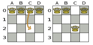
The new solution is called a neighbor of the original solution, because it can be reached in a single Move.
Although a single move can change multiple queens, the neighbors of a solution should always be a very small subset of all possible solutions.
For example, on that original solution, these are all possible changeMoves:
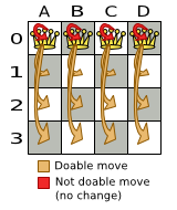
If we ignore the four changeMoves that have no impact and are therefore not doable, we can see that the number of moves is n * (n - 1) = 12.
This is far less than the number of possible solutions, which is n ^ n = 256.
As the problem scales out, the number of possible moves increases far less than the number of possible solutions.
Yet, in four changeMoves or less we can reach any solution.
For example we can reach a very different solution in three changeMoves:
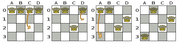
|
There are many other types of moves besides A |
All optimization algorithms use Moves to transition from one solution to a neighbor solution.
Therefore, all the optimization algorithms are confronted with Move selection: the craft of creating and iterating moves efficiently and the art of finding the most promising subset of random moves to evaluate first.
10.1.2. What is a MoveSelector?
A MoveSelector's main function is to create Iterator<Move> when needed.
An optimization algorithm will iterate through a subset of those moves.
Here’s an example how to configure a changeMoveSelector for the optimization algorithm Local Search:
<localSearch>
<changeMoveSelector/>
...
</localSearch>Out of the box, this works and all properties of the changeMoveSelector are defaulted sensibly (unless that fails fast due to ambiguity). On the other hand, the configuration can be customized significantly for specific use cases.
For example: you might want to configure a filter to discard pointless moves.
10.1.3. Subselecting of entities, values, and other moves
To create a Move, a MoveSelector needs to select one or more planning entities and/or planning values to move.
Just like MoveSelectors, EntitySelectors and ValueSelectors need to support a similar feature set (such as scalable just-in-time selection). Therefore, they all implement a common interface Selector and they are configured similarly.
A MoveSelector is often composed out of EntitySelectors, ValueSelectors or even other MoveSelectors, which can be configured individually if desired:
<unionMoveSelector>
<changeMoveSelector>
<entitySelector>
...
</entitySelector>
<valueSelector>
...
</valueSelector>
...
</changeMoveSelector>
<swapMoveSelector>
...
</swapMoveSelector>
</unionMoveSelector>Together, this structure forms a Selector tree:
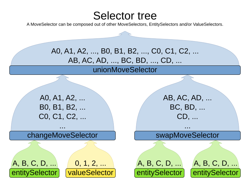
The root of this tree is a MoveSelector which is injected into the optimization algorithm implementation to be (partially) iterated in every step.
10.2. Generic MoveSelectors
10.2.1. Generic MoveSelectors overview
| Name | Description | toString() example |
|---|---|---|
Change 1 entity’s variable |
|
|
Swap all variables of 2 entities |
|
|
Change a set of entities with the same value |
|
|
Swap 2 sets of entities with the same values |
|
|
Move a list element to a different index or to another entity’s list variable |
|
|
Swap 2 list elements |
|
|
Move a subList from one position to another |
|
|
Swap 2 subLists |
|
|
Select an entity, remove k edges from its list variable, add k new edges from the removed endpoints |
|
|
Swap 2 tails chains |
|
|
Cut a subchain and paste it into another chain |
|
|
Swap 2 subchains |
|
10.2.2. ChangeMoveSelector
For one planning variable, the ChangeMove selects one planning entity and one planning value and assigns the entity’s variable to that value.
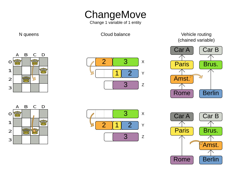
Simplest configuration:
<changeMoveSelector/>If there are multiple entity classes or multiple planning variables for one entity class, a simple configuration will automatically unfold into a union of ChangeMove selectors for every planning variable.
Advanced configuration:
<changeMoveSelector>
... <!-- Normal selector properties -->
<entitySelector>
<entityClass>...Lecture</entityClass>
...
</entitySelector>
<valueSelector variableName="room">
...
<nearbySelection>...</nearbySelection>
</valueSelector>
</changeMoveSelector>A ChangeMove is the finest grained move.
|
Almost every |
This move selector only supports phase or solver caching if it doesn’t apply on a chained variable.
10.2.3. SwapMoveSelector
The SwapMove selects two different planning entities and swaps the planning values of all their planning variables.
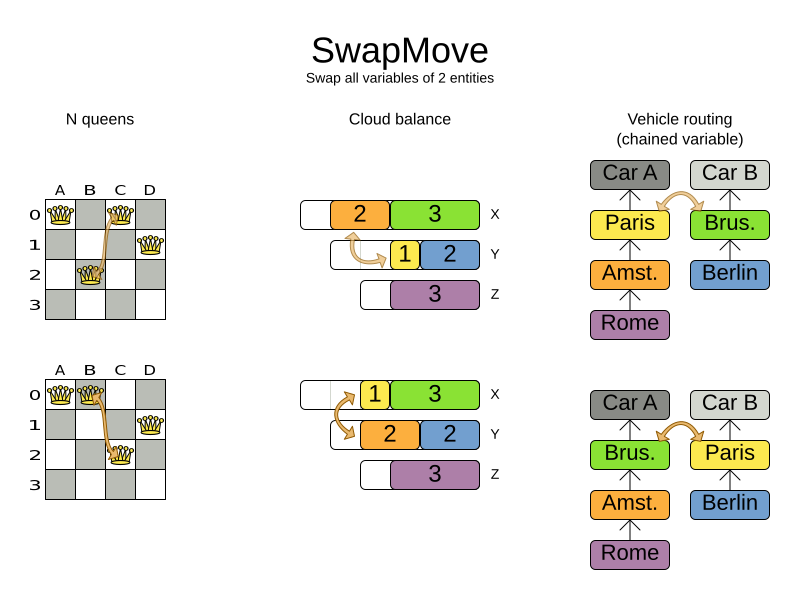
Although a SwapMove on a single variable is essentially just two ChangeMoves,
it’s often the winning step in cases that the first of the two ChangeMoves would not win
because it leaves the solution in a state with broken hard constraints.
For example: swapping the room of two lectures doesn’t bring the solution in an intermediate state where both lectures are in the same room which breaks a hard constraint.
Simplest configuration:
<swapMoveSelector/>If there are multiple entity classes, a simple configuration will automatically unfold into a union of SwapMove selectors for every entity class.
Advanced configuration:
<swapMoveSelector>
... <!-- Normal selector properties -->
<entitySelector>
<entityClass>...Lecture</entityClass>
...
</entitySelector>
<secondaryEntitySelector>
<entityClass>...Lecture</entityClass>
...
<nearbySelection>...</nearbySelection>
</secondaryEntitySelector>
<variableNameIncludes>
<variableNameInclude>room</variableNameInclude>
<variableNameInclude>...</variableNameInclude>
</variableNameIncludes>
</swapMoveSelector>The secondaryEntitySelector is rarely needed: if it is not specified, entities from the same entitySelector are swapped.
If one or more variableNameInclude properties are specified, not all planning variables will be swapped, but only those specified.
For example for course scheduling, specifying only variableNameInclude room will make it only swap room, not period.
This move selector only supports phase or solver caching if it doesn’t apply on any chained variables.
10.2.4. Pillar-based move selectors
A pillar is a set of planning entities which have the same planning value(s) for their planning variable(s).
10.2.4.1. PillarChangeMoveSelector
The PillarChangeMove selects one entity pillar (or subset of those) and changes the value of one variable (which is the same for all entities) to another value.
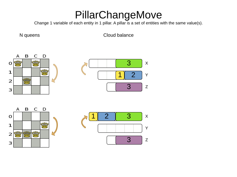
In the example above, queen A and C have the same value (row 0) and are moved to row 2. Also the yellow and blue process have the same value (computer Y) and are moved to computer X.
Simplest configuration:
<pillarChangeMoveSelector/>Advanced configuration:
<pillarChangeMoveSelector>
<subPillarType>SEQUENCE</subPillarType>
<subPillarSequenceComparatorClass>org.optaplanner.examples.nurserostering.domain.ShiftAssignmentComparator</subPillarSequenceComparatorClass>
... <!-- Normal selector properties -->
<pillarSelector>
<entitySelector>
<entityClass>...ShiftAssignment</entityClass>
...
</entitySelector>
<minimumSubPillarSize>1</minimumSubPillarSize>
<maximumSubPillarSize>1000</maximumSubPillarSize>
</pillarSelector>
<valueSelector variableName="room">
...
</valueSelector>
</pillarChangeMoveSelector>For a description of subPillarType and related properties, please refer to Subpillars.
The other properties are explained in changeMoveSelector. This move selector does not support phase or solver caching and step caching scales badly memory wise.
10.2.4.2. PillarSwapMoveSelector
The PillarSwapMove selects two different entity pillars and swaps the values of all their variables for all their entities.
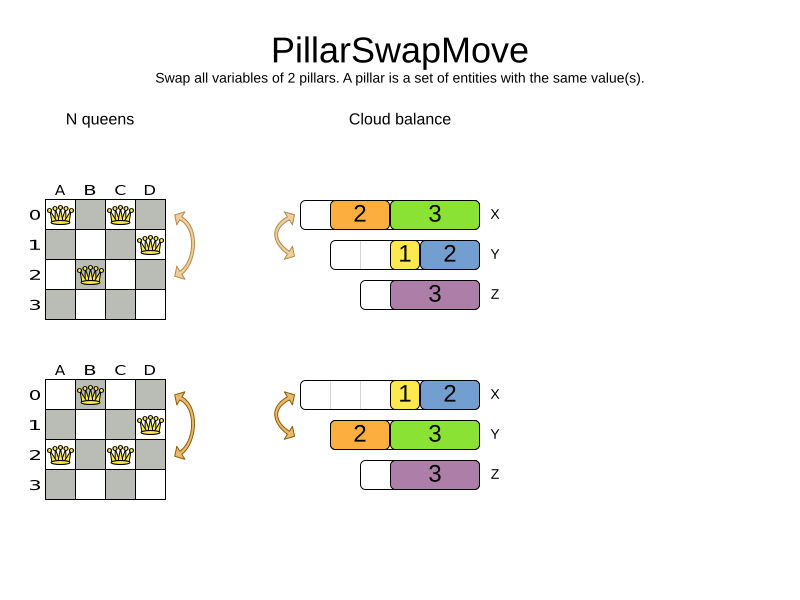
Simplest configuration:
<pillarSwapMoveSelector/>Advanced configuration:
<pillarSwapMoveSelector>
<subPillarType>SEQUENCE</subPillarType>
<subPillarSequenceComparatorClass>org.optaplanner.examples.nurserostering.domain.ShiftAssignmentComparator</subPillarSequenceComparatorClass>
... <!-- Normal selector properties -->
<pillarSelector>
<entitySelector>
<entityClass>...ShiftAssignment</entityClass>
...
</entitySelector>
<minimumSubPillarSize>1</minimumSubPillarSize>
<maximumSubPillarSize>1000</maximumSubPillarSize>
</pillarSelector>
<secondaryPillarSelector>
<entitySelector>
...
</entitySelector>
...
</secondaryPillarSelector>
<variableNameIncludes>
<variableNameInclude>employee</variableNameInclude>
<variableNameInclude>...</variableNameInclude>
</variableNameIncludes>
</pillarSwapMoveSelector>For a description of subPillarType and related properties, please refer to sub pillars.
The secondaryPillarSelector is rarely needed: if it is not specified, entities from the same pillarSelector are swapped.
The other properties are explained in swapMoveSelector and pillarChangeMoveSelector. This move selector does not support phase or solver caching and step caching scales badly memory wise.
10.2.4.3. Sub pillars
A sub pillar is a subset of entities that share the same value(s) for their variable(s). For example if queen A, B, C and D are all located on row 0, they are a pillar and [A, D] is one of the many sub pillars.
There are several ways how sub pillars can be selected by the subPillarType property:
-
ALL(default) selects all possible sub pillars. -
SEQUENCElimits selection of sub pillars to Sequential sub pillars. -
NONEnever selects any sub pillars.
If sub pillars are enabled, the pillar itself is also included and the properties minimumSubPillarSize (defaults to 1) and maximumSubPillarSize (defaults to infinity) limit the size of the selected (sub) pillar.
|
The number of sub pillars of a pillar is exponential to the size of the pillar.
For example a pillar of size 32 has |
10.2.4.3.1. Sequential sub pillars
Sub pillars can be sorted with a Comparator. A sequential sub pillar is a continuous subset of its sorted base pillar.
For example if a nurse has shifts on Monday (M), Tuesday (T), and Wednesday (W), they are a pillar and only the following are its sequential sub pillars: [M], [T], [W], [M, T], [T, W], [M, T, W].
But [M, W] is not a sub pillar in this case, as there is a gap on Tuesday.
Sequential sub pillars apply to both Pillar change move and Pillar swap move. A minimal configuration looks like this:
<pillar...MoveSelector>
<subPillarType>SEQUENCE</subPillarType>
</pillar...MoveSelector>In this case, the entity being operated on must implement the Comparable interface. The size of sub pillars will not be limited in any way.
An advanced configuration looks like this:
<pillar...MoveSelector>
...
<subPillarType>SEQUENCE</subPillarType>
<subPillarSequenceComparatorClass>org.optaplanner.examples.nurserostering.domain.ShiftAssignmentComparator</subPillarSequenceComparatorClass>
<pillarSelector>
...
<minimumSubPillarSize>1</minimumSubPillarSize>
<maximumSubPillarSize>1000</maximumSubPillarSize>
</pillarSelector>
...
</pillar...MoveSelector>In this case, the entity being operated on need not be Comparable. The given subPillarSequenceComparatorClass is used to establish the sequence instead. Also, the size of the sub pillars is limited in length of up to 1000 entities.
10.2.5. Move selectors for list variables
10.2.5.1. ListChangeMoveSelector
The ListChangeMoveSelector selects an element from a list variable’s value range and moves it from its current position to a new one.
Simplest configuration:
<listChangeMoveSelector/>Advanced configuration:
<listChangeMoveSelector>
... <!-- Normal selector properties -->
<valueSelector id="valueSelector1">
...
</valueSelector>
<destinationSelector>
<entitySelector>
...
</entitySelector>
<valueSelector>
...
</valueSelector>
<nearbySelection>
<originValueSelector mimicSelectorRef="valueSelector1"/>
... <!-- Normal nearby selection properties -->
</nearbySelection>
</destinationSelector>
</listChangeMoveSelector>10.2.5.2. ListSwapMoveSelector
The ListSwapMoveSelector selects two elements from the same list variable value range and swaps their positions.
Simplest configuration:
<listSwapMoveSelector/>Advanced configuration:
<listSwapMoveSelector>
... <!-- Normal selector properties -->
<valueSelector id="valueSelector1">
...
</valueSelector>
<secondaryValueSelector>
<nearbySelection>
<originValueSelector mimicSelectorRef="valueSelector1"/>
... <!-- Normal nearby selection properties -->
</nearbySelection>
</secondaryValueSelector>
</listSwapMoveSelector>10.2.5.3. SubListChangeMoveSelector
A subList is a sequence of elements in a specific entity’s list variable between fromIndex and toIndex.
The SubListChangeMoveSelector selects a source subList by selecting a source entity and the source subList’s fromIndex and toIndex.
Then it selects a destination entity and a destinationIndex in the destination entity’s list variable.
Selecting these parameters results in a SubListChangeMove that removes the source subList elements from the source entity and adds them to the destination entity’s list variable at the destinationIndex.
Simplest configuration:
<subListChangeMoveSelector/>Advanced configuration:
<subListChangeMoveSelector>
... <!-- Normal selector properties -->
<selectReversingMoveToo>true</selectReversingMoveToo>
<subListSelector id="subListSelector1">
<valueSelector>
...
</valueSelector>
<minimumSubListSize>2</minimumSubListSize>
<maximumSubListSize>6</maximumSubListSize>
</subListSelector>
<destinationSelector>
<entitySelector>
...
</entitySelector>
<valueSelector>
...
</valueSelector>
<nearbySelection>
<originSubListSelector mimicSelectorRef="subListSelector1"/>
... <!-- Normal nearby selection properties -->
</nearbySelection>
</destinationSelector>
</subListChangeMoveSelector>10.2.5.4. SubListSwapMoveSelector
A subList is a sequence of elements in a specific entity’s list variable between fromIndex and toIndex.
The SubListSwapMoveSelector selects a left subList by selecting a left entity and the left subList’s fromIndex and toIndex.
Then it selects a right subList by selecting a right entity and the right subList’s fromIndex and toIndex.
Selecting these parameters results in a SubListSwapMove that swaps the right and left subLists between right and left entities.
Simplest configuration:
<subListSwapMoveSelector/>Advanced configuration:
<subListSwapMoveSelector>
... <!-- Normal selector properties -->
<selectReversingMoveToo>true</selectReversingMoveToo>
<subListSelector id="subListSelector1">
<valueSelector>
...
</valueSelector>
<minimumSubListSize>2</minimumSubListSize>
<maximumSubListSize>6</maximumSubListSize>
</subListSelector>
<secondarySubListSelector>
<valueSelector>
...
</valueSelector>
<nearbySelection>
<originSubListSelector mimicSelectorRef="subListSelector1"/>
... <!-- Normal nearby selection properties -->
</nearbySelection>
<minimumSubListSize>3</minimumSubListSize>
<maximumSubListSize>5</maximumSubListSize>
</secondarySubListSelector>
</subListSwapMoveSelector>10.2.5.5. KOptListMoveSelector
The KOptListMoveSelector considers the list variable to be
a graph whose edges are the consecutive elements of the list
(with the last element being consecutive to the first element).
A KOptListMove selects an entity, remove k edges from its list variable, and add k new edges from the removed edges' endpoints.
This move may reverse segments of the graph.
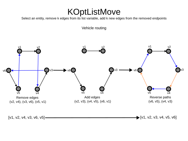
Simplest configuration:
<kOptListMoveSelector/>Advanced configuration:
<kOptListMoveSelector>
... <!-- Normal selector properties -->
<minimumK>2</minimumK>
<maximumK>4</maximumK>
</kOptListMoveSelector>10.2.6. Move selectors for chained variables
10.2.6.1. TailChainSwapMoveSelector or 2-opt
A tailChain is a set of planning entities with a chained planning variable which form the last part of a chain.
The tailChainSwapMove selects a tail chain and swaps it with the tail chain of another planning value (in a different or the same anchor chain). If the targeted planning value, doesn’t have a tail chain, it swaps with nothing (resulting in a change like move). If it occurs within the same anchor chain, a partial chain reverse occurs.
In academic papers, this is often called a 2-opt move.
Simplest configuration:
<tailChainSwapMoveSelector/>Advanced configuration:
<tailChainSwapMoveSelector>
... <!-- Normal selector properties -->
<entitySelector>
<entityClass>...Customer</entityClass>
...
</entitySelector>
<valueSelector variableName="previousStandstill">
...
<nearbySelection>...</nearbySelection>
</valueSelector>
</tailChainSwapMoveSelector>The entitySelector selects the start of the tail chain that is being moved.
The valueSelector selects to where that tail chain is moved.
If it has a tail chain itself, that is moved to the location of the original tail chain.
It uses a valueSelector instead of a secondaryEntitySelector to be able to include all possible 2opt moves (such as moving to the end of a tail) and to work correctly with nearby selection (because of asymmetric distances and also swapped entity distance gives an incorrect selection probability).
|
Although |
This move selector does not support phase or solver caching.
10.2.6.2. SubChainChangeMoveSelector
A subChain is a set of planning entities with a chained planning variable which form part of a chain.
The subChainChangeMoveSelector selects a subChain and moves it to another place (in a different or the same anchor chain).
Simplest configuration:
<subChainChangeMoveSelector/>Advanced configuration:
<subChainChangeMoveSelector>
... <!-- Normal selector properties -->
<entityClass>...Customer</entityClass>
<subChainSelector>
<valueSelector variableName="previousStandstill">
...
</valueSelector>
<minimumSubChainSize>2</minimumSubChainSize>
<maximumSubChainSize>40</maximumSubChainSize>
</subChainSelector>
<valueSelector variableName="previousStandstill">
...
</valueSelector>
<selectReversingMoveToo>true</selectReversingMoveToo>
</subChainChangeMoveSelector>The subChainSelector selects a number of entities, no less than minimumSubChainSize (defaults to 1) and no more than maximumSubChainSize (defaults to infinity).
|
If Furthermore, in a |
The selectReversingMoveToo property (defaults to true) enables selecting the reverse of every subchain too.
This move selector does not support phase or solver caching and step caching scales badly memory wise.
10.2.6.3. SubChainSwapMoveSelector
The subChainSwapMoveSelector selects two different subChains and moves them to another place in a different or the same anchor chain.
Simplest configuration:
<subChainSwapMoveSelector/>Advanced configuration:
<subChainSwapMoveSelector>
... <!-- Normal selector properties -->
<entityClass>...Customer</entityClass>
<subChainSelector>
<valueSelector variableName="previousStandstill">
...
</valueSelector>
<minimumSubChainSize>2</minimumSubChainSize>
<maximumSubChainSize>40</maximumSubChainSize>
</subChainSelector>
<secondarySubChainSelector>
<valueSelector variableName="previousStandstill">
...
</valueSelector>
<minimumSubChainSize>2</minimumSubChainSize>
<maximumSubChainSize>40</maximumSubChainSize>
</secondarySubChainSelector>
<selectReversingMoveToo>true</selectReversingMoveToo>
</subChainSwapMoveSelector>The secondarySubChainSelector is rarely needed: if it is not specified, entities from the same subChainSelector are swapped.
The other properties are explained in subChainChangeMoveSelector. This move selector does not support phase or solver caching and step caching scales badly memory wise.
10.3. Combining multiple MoveSelectors
10.3.1. unionMoveSelector
A unionMoveSelector selects a Move by selecting one of its MoveSelector children to supply the next Move.
Simplest configuration:
<unionMoveSelector>
<...MoveSelector/>
<...MoveSelector/>
<...MoveSelector/>
...
</unionMoveSelector>Advanced configuration:
<unionMoveSelector>
... <!-- Normal selector properties -->
<changeMoveSelector>
<fixedProbabilityWeight>...</fixedProbabilityWeight>
...
</changeMoveSelector>
<swapMoveSelector>
<fixedProbabilityWeight>...</fixedProbabilityWeight>
...
</swapMoveSelector>
<...MoveSelector>
<fixedProbabilityWeight>...</fixedProbabilityWeight>
...
</...MoveSelector>
...
<selectorProbabilityWeightFactoryClass>...ProbabilityWeightFactory</selectorProbabilityWeightFactoryClass>
</unionMoveSelector>The selectorProbabilityWeightFactory determines in selectionOrder RANDOM how often a MoveSelector child is selected to supply the next Move.
By default, each MoveSelector child has the same chance of being selected.
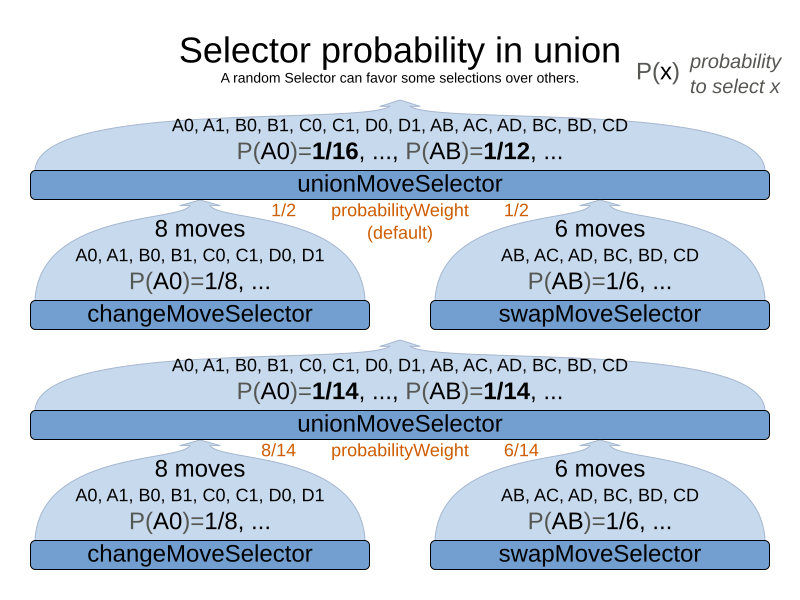
Change the fixedProbabilityWeight of such a child to select it more often.
For example, the unionMoveSelector can return a SwapMove twice as often as a ChangeMove:
<unionMoveSelector>
<changeMoveSelector>
<fixedProbabilityWeight>1.0</fixedProbabilityWeight>
...
</changeMoveSelector>
<swapMoveSelector>
<fixedProbabilityWeight>2.0</fixedProbabilityWeight>
...
</swapMoveSelector>
</unionMoveSelector>The number of possible ChangeMoves is very different from the number of possible SwapMoves and furthermore it’s problem dependent.
To give each individual Move the same selection chance (as opposed to each MoveSelector), use the FairSelectorProbabilityWeightFactory:
<unionMoveSelector>
<changeMoveSelector/>
<swapMoveSelector/>
<selectorProbabilityWeightFactoryClass>org.optaplanner.core.impl.heuristic.selector.common.decorator.FairSelectorProbabilityWeightFactory</selectorProbabilityWeightFactoryClass>
</unionMoveSelector>10.3.2. cartesianProductMoveSelector
A cartesianProductMoveSelector selects a new CompositeMove.
It builds that CompositeMove by selecting one Move per MoveSelector child and adding it to the CompositeMove.
Simplest configuration:
<cartesianProductMoveSelector>
<...MoveSelector/>
<...MoveSelector/>
<...MoveSelector/>
...
</cartesianProductMoveSelector>Advanced configuration:
<cartesianProductMoveSelector>
... <!-- Normal selector properties -->
<changeMoveSelector>
...
</changeMoveSelector>
<swapMoveSelector>
...
</swapMoveSelector>
<...MoveSelector>
...
</...MoveSelector>
...
<ignoreEmptyChildIterators>true</ignoreEmptyChildIterators>
</cartesianProductMoveSelector>The ignoreEmptyChildIterators property (true by default) will ignore every empty childMoveSelector to avoid returning no moves.
For example: a cartesian product of changeMoveSelector A and B, for which B is empty (because all it’s entities are pinned) returns no move if ignoreEmptyChildIterators is false and the moves of A if ignoreEmptyChildIterators is true.
To enforce that two child selectors use the same entity or value efficiently, use mimic selection, not move filtering.
10.4. EntitySelector
Simplest configuration:
<entitySelector/>Advanced configuration:
<entitySelector>
... <!-- Normal selector properties -->
<entityClass>org.optaplanner.examples.curriculumcourse.domain.Lecture</entityClass>
</entitySelector>The entityClass property is only required if it cannot be deduced automatically because there are multiple entity classes.
10.5. ValueSelector
Simplest configuration:
<valueSelector/>Advanced configuration:
<valueSelector variableName="room">
... <!-- Normal selector properties -->
</valueSelector>The variableName property is only required if it cannot be deduced automatically because there are multiple variables (for the related entity class).
In exotic Construction Heuristic configurations, the entityClass from the EntitySelector sometimes needs to be downcasted, which can be done with the property downcastEntityClass:
<valueSelector variableName="period">
<downcastEntityClass>...LeadingExam</downcastEntityClass>
</valueSelector>If a selected entity cannot be downcasted, the ValueSelector is empty for that entity.
10.6. General Selector features
10.6.1. CacheType: create moves ahead of time or just in time
A Selector's cacheType determines when a selection (such as a Move, an entity, a value, …)
is created and how long it lives.
Almost every Selector supports setting a cacheType:
<changeMoveSelector>
<cacheType>PHASE</cacheType>
...
</changeMoveSelector>The following cacheTypes are supported:
-
JUST_IN_TIME(default, recommended): Not cached. Construct each selection (Move, …) just before it’s used. This scales up well in memory footprint. -
STEP: Cached. Create each selection (Move, …) at the beginning of a step and cache them in a list for the remainder of the step. This scales up badly in memory footprint. -
PHASE: Cached. Create each selection (Move, …) at the beginning of a solver phase and cache them in a list for the remainder of the phase. Some selections cannot be phase cached because the list changes every step. This scales up badly in memory footprint, but has a slight performance gain. -
SOLVER: Cached. Create each selection (Move, …) at the beginning of aSolverand cache them in a list for the remainder of theSolver. Some selections cannot be solver cached because the list changes every step. This scales up badly in memory footprint, but has a slight performance gain.
A cacheType can be set on composite selectors too:
<unionMoveSelector>
<cacheType>PHASE</cacheType>
<changeMoveSelector/>
<swapMoveSelector/>
...
</unionMoveSelector>Nested selectors of a cached selector cannot be configured to be cached themselves, unless it’s a higher cacheType.
For example: a STEP cached unionMoveSelector can contain a PHASE cached changeMoveSelector,
but it cannot contain a STEP cached changeMoveSelector.
10.6.2. SelectionOrder: original, sorted, random, shuffled, or probabilistic
A Selector's selectionOrder determines the order in which the selections (such as Moves, entities, values, …) are iterated.
An optimization algorithm will usually only iterate through a subset of its MoveSelector's selections, starting from the start, so the selectionOrder is critical to decide which Moves are actually evaluated.
Almost every Selector supports setting a selectionOrder:
<changeMoveSelector>
...
<selectionOrder>RANDOM</selectionOrder>
...
</changeMoveSelector>The following selectionOrders are supported:
-
ORIGINAL: Select the selections (Moves, entities, values, …) in default order. Each selection will be selected only once.-
For example: A0, A1, A2, A3, …, B0, B1, B2, B3, …, C0, C1, C2, C3, …
-
-
SORTED: Select the selections (
Moves, entities, values, …) in sorted order. Each selection will be selected only once. RequirescacheType >= STEP. Mostly used on anentitySelectororvalueSelectorfor construction heuristics. See sorted selection.-
For example: A0, B0, C0, …, A2, B2, C2, …, A1, B1, C1, …
-
-
RANDOM (default): Select the selections (
Moves, entities, values, …) in non-shuffled random order. A selection might be selected multiple times. This scales up well in performance because it does not require caching.-
For example: C2, A3, B1, C2, A0, C0, …
-
-
SHUFFLED: Select the selections (
Moves, entities, values, …) in shuffled random order. Each selection will be selected only once. RequirescacheType >= STEP. This scales up badly in performance, not just because it requires caching, but also because a random number is generated for each element, even if it’s not selected (which is the grand majority when scaling up).-
For example: C2, A3, B1, A0, C0, …
-
-
PROBABILISTIC: Select the selections (
Moves, entities, values, …) in random order, based on the selection probability of each element. A selection with a higher probability has a higher chance to be selected than elements with a lower probability. A selection might be selected multiple times. RequirescacheType >= STEP. Mostly used on anentitySelectororvalueSelector. See probabilistic selection.-
For example: B1, B1, A1, B2, B1, C2, B1, B1, …
-
A selectionOrder can be set on composite selectors too.
|
When a |
10.6.3. Recommended combinations of CacheType and SelectionOrder
10.6.3.1. Just in time random selection (default)
This combination is great for big use cases (10 000 entities or more), as it scales up well in memory footprint and performance.
Other combinations are often not even viable on such sizes.
It works for smaller use cases too, so it’s a good way to start out.
It’s the default, so this explicit configuration of cacheType and selectionOrder is actually obsolete:
<unionMoveSelector>
<cacheType>JUST_IN_TIME</cacheType>
<selectionOrder>RANDOM</selectionOrder>
<changeMoveSelector/>
<swapMoveSelector/>
</unionMoveSelector>Here’s how it works.
When Iterator<Move>.next() is called, a child MoveSelector is randomly selected (1), which creates a random Move (2, 3, 4) and is then returned (5):
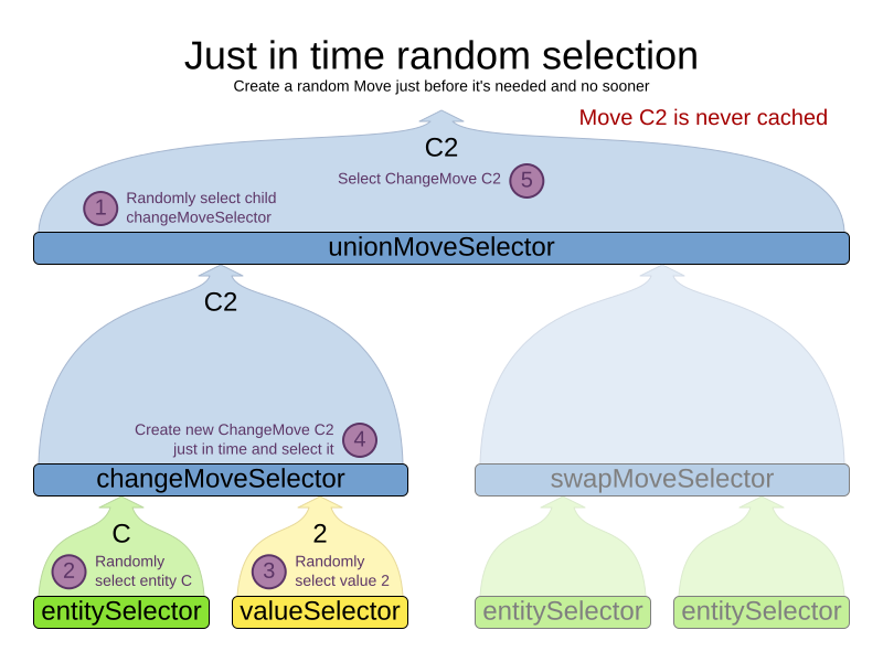
Notice that it never creates a list of Moves and it generates random numbers only for Moves that are actually selected.
10.6.3.2. Cached shuffled selection
This combination often wins for small use cases (1000 entities or less). Beyond that size, it scales up badly in memory footprint and performance.
<unionMoveSelector>
<cacheType>PHASE</cacheType>
<selectionOrder>SHUFFLED</selectionOrder>
<changeMoveSelector/>
<swapMoveSelector/>
</unionMoveSelector>Here’s how it works: At the start of the phase (or step depending on the cacheType), all moves are created (1) and cached (2). When MoveSelector.iterator() is called, the moves are shuffled (3). When Iterator<Move>.next() is called, the next element in the shuffled list is returned (4):
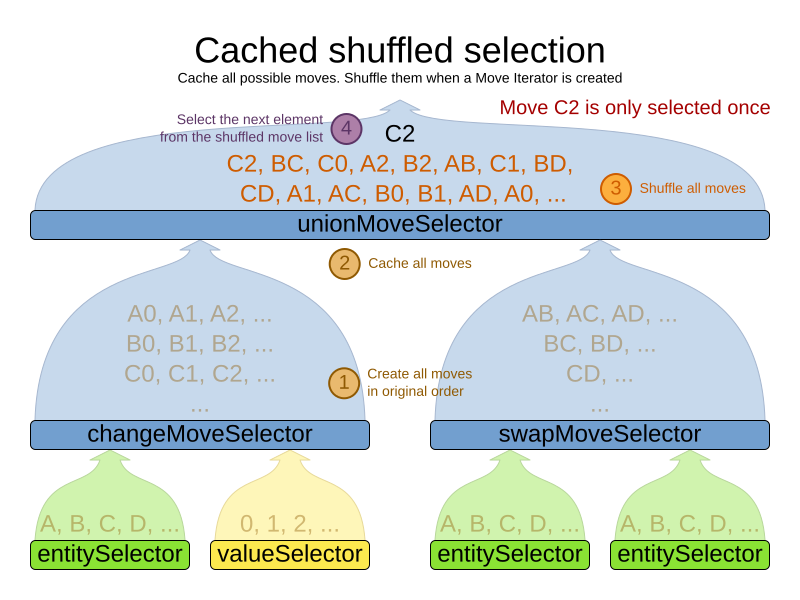
Notice that each Move will only be selected once, even though they are selected in random order.
Use cacheType PHASE if none of the (possibly nested) Selectors require STEP.
Otherwise, do something like this:
<unionMoveSelector>
<cacheType>STEP</cacheType>
<selectionOrder>SHUFFLED</selectionOrder>
<changeMoveSelector>
<cacheType>PHASE</cacheType>
</changeMoveSelector>
<swapMoveSelector>
<cacheType>PHASE</cacheType>
</swapMoveSelector>
<pillarSwapMoveSelector/><!-- Does not support cacheType PHASE -->
</unionMoveSelector>10.6.3.3. Cached random selection
This combination is often a worthy competitor for medium use cases, especially with fast stepping optimization algorithms (such as Simulated Annealing). Unlike cached shuffled selection, it doesn’t waste time shuffling the moves list at the beginning of every step.
<unionMoveSelector>
<cacheType>PHASE</cacheType>
<selectionOrder>RANDOM</selectionOrder>
<changeMoveSelector/>
<swapMoveSelector/>
</unionMoveSelector>10.6.4. Filtered selection
There can be certain moves that you don’t want to select, because:
-
The move is pointless and would only waste CPU time. For example, swapping two lectures of the same course will result in the same score and the same schedule because all lectures of one course are interchangeable (same teacher, same students, same topic).
-
Doing the move would break a built-in hard constraint, so the solution would be infeasible but the score function doesn’t check built-in hard constraints for performance reasons. For example, don’t change a gym lecture to a room which is not a gym room. It’s usually better to not use move filtering for such cases, because it allows the metaheuristics to temporarily break hard constraints to escape local optima.
Any built-in hard constraint must probably be filtered on every move type of every solver phase. For example if it filters the change move of Local Search, it must also filter the swap move that swaps the room of a gym lecture with another lecture for which the other lecture’s original room isn’t a gym room. Furthermore, it must also filter the change moves of the Construction Heuristics (which requires an advanced configuration).
If a move is unaccepted by the filter, it’s not executed and the score isn’t calculated.
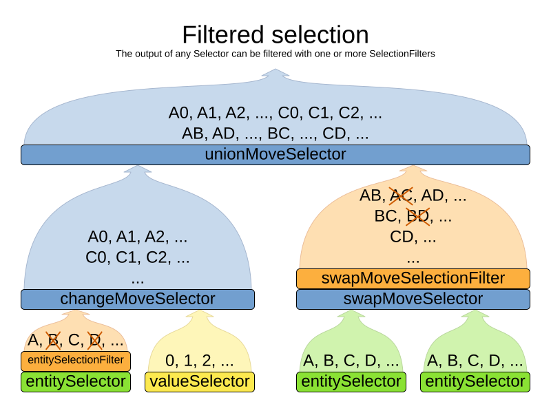
Filtering uses the interface SelectionFilter:
public interface SelectionFilter<Solution_, T> {
boolean accept(ScoreDirector<Solution_> scoreDirector, T selection);
}Implement the accept method to return false on a discarded selection (see below).
Filtered selection can happen on any Selector in the selector tree, including any MoveSelector, EntitySelector
or ValueSelector.
It works with any cacheType and selectionOrder.
|
Apply the filter on the lowest level possible. In most cases, you’ll need to know both the entity and the value involved so you’ll have to apply it on the move selector. |
|
|
10.6.4.1. Filtered move selection
Unaccepted moves will not be selected and will therefore never have their doMove() method called:
public class DifferentCourseSwapMoveFilter implements SelectionFilter<CourseSchedule, SwapMove> {
@Override
public boolean accept(ScoreDirector<CourseSchedule> scoreDirector, SwapMove move) {
Lecture leftLecture = (Lecture) move.getLeftEntity();
Lecture rightLecture = (Lecture) move.getRightEntity();
return !leftLecture.getCourse().equals(rightLecture.getCourse());
}
}Configure the filterClass on every targeted moveSelector (potentially both in the Local Search and the Construction Heuristics if it filters ChangeMoves):
<swapMoveSelector>
<filterClass>org.optaplanner.examples.curriculumcourse.solver.move.DifferentCourseSwapMoveFilter</filterClass>
</swapMoveSelector>10.6.4.2. Filtered entity selection
Unaccepted entities will not be selected and will therefore never be used to create a move.
public class LongLectureSelectionFilter implements SelectionFilter<CourseSchedule, Lecture> {
@Override
public boolean accept(ScoreDirector<CourseSchedule> scoreDirector, Lecture lecture) {
return lecture.isLong();
}
}Configure the filterClass on every targeted entitySelector (potentially both in the Local Search and the Construction Heuristics):
<changeMoveSelector>
<entitySelector>
<filterClass>org.optaplanner.examples.curriculumcourse.solver.move.LongLectureSelectionFilter</filterClass>
</entitySelector>
</changeMoveSelector>If that filter should apply on all entities, configure it as a global pinningFilter instead.
10.6.4.3. Filtered value selection
Unaccepted values will not be selected and will therefore never be used to create a move.
public class LongPeriodSelectionFilter implements SelectionFilter<CourseSchedule, Period> {
@Override
public boolean accept(ScoreDirector<CourseSchedule> scoreDirector, Period period) {
return period();
}
}Configure the filterClass on every targeted valueSelector (potentially both in the Local Search and the Construction Heuristics):
<changeMoveSelector>
<valueSelector>
<filterClass>org.optaplanner.examples.curriculumcourse.solver.move.LongPeriodSelectionFilter</filterClass>
</valueSelector>
</changeMoveSelector>10.6.5. Sorted selection
Sorted selection can happen on any Selector in the selector tree, including any MoveSelector, EntitySelector or ValueSelector.
It does not work with cacheType JUST_IN_TIME and it only works with selectionOrder SORTED.
It’s mostly used in construction heuristics.
|
If the chosen construction heuristic implies sorting, for example |
10.6.5.1. Sorted selection by SorterManner
Some Selector types implement a SorterManner out of the box:
-
EntitySelectorsupports:-
DECREASING_DIFFICULTY: Sorts the planning entities according to decreasing planning entity difficulty. Requires that planning entity difficulty is annotated on the domain model.<entitySelector> <cacheType>PHASE</cacheType> <selectionOrder>SORTED</selectionOrder> <sorterManner>DECREASING_DIFFICULTY</sorterManner> </entitySelector>
-
-
ValueSelectorsupports:-
INCREASING_STRENGTH: Sorts the planning values according to increasing planning value strength. Requires that planning value strength is annotated on the domain model.<valueSelector> <cacheType>PHASE</cacheType> <selectionOrder>SORTED</selectionOrder> <sorterManner>INCREASING_STRENGTH</sorterManner> </valueSelector>
-
10.6.5.2. Sorted selection by Comparator
An easy way to sort a Selector is with a plain old Comparator:
public class CloudProcessDifficultyComparator implements Comparator<CloudProcess> {

    public int compare(CloudProcess a, CloudProcess b) {
        return new CompareToBuilder()
                .append(a.getRequiredMultiplicand(), b.getRequiredMultiplicand())
                .append(a.getId(), b.getId())
                .toComparison();
    }

}You’ll also need to configure it (unless it’s annotated on the domain model and automatically applied by the optimization algorithm):
<entitySelector>
<cacheType>PHASE</cacheType>
<selectionOrder>SORTED</selectionOrder>
<sorterComparatorClass>...CloudProcessDifficultyComparator</sorterComparatorClass>
<sorterOrder>DESCENDING</sorterOrder>
</entitySelector>|
|
10.6.5.3. Sorted selection by SelectionSorterWeightFactory
If you need the entire solution to sort a Selector, use a SelectionSorterWeightFactory instead:
public interface SelectionSorterWeightFactory<Solution_, T> {
Comparable createSorterWeight(Solution_ solution, T selection);
}public class QueenDifficultyWeightFactory implements SelectionSorterWeightFactory<NQueens, Queen> {
public QueenDifficultyWeight createSorterWeight(NQueens nQueens, Queen queen) {
int distanceFromMiddle = calculateDistanceFromMiddle(nQueens.getN(), queen.getColumnIndex());
return new QueenDifficultyWeight(queen, distanceFromMiddle);
}
...
public static class QueenDifficultyWeight implements Comparable<QueenDifficultyWeight> {
private final Queen queen;
private final int distanceFromMiddle;
public QueenDifficultyWeight(Queen queen, int distanceFromMiddle) {
this.queen = queen;
this.distanceFromMiddle = distanceFromMiddle;
}
public int compareTo(QueenDifficultyWeight other) {
return new CompareToBuilder()
// The more difficult queens have a lower distance to the middle
.append(other.distanceFromMiddle, distanceFromMiddle) // Decreasing
// Tie breaker
.append(queen.getColumnIndex(), other.queen.getColumnIndex())
.toComparison();
}
}
}You’ll also need to configure it (unless it’s annotated on the domain model and automatically applied by the optimization algorithm):
<entitySelector>
<cacheType>PHASE</cacheType>
<selectionOrder>SORTED</selectionOrder>
<sorterWeightFactoryClass>...QueenDifficultyWeightFactory</sorterWeightFactoryClass>
<sorterOrder>DESCENDING</sorterOrder>
</entitySelector>|
|
10.6.5.4. Sorted selection by SelectionSorter
Alternatively, you can also use the interface SelectionSorter directly:
public interface SelectionSorter<Solution_, T> {
void sort(ScoreDirector<Solution_> scoreDirector, List<T> selectionList);
} <entitySelector>
<cacheType>PHASE</cacheType>
<selectionOrder>SORTED</selectionOrder>
<sorterClass>...MyEntitySorter</sorterClass>
</entitySelector>|
|
10.6.6. Probabilistic selection
Probabilistic selection can happen on any Selector in the selector tree, including any MoveSelector, EntitySelector or ValueSelector.
It does not work with cacheType JUST_IN_TIME and it only works with selectionOrder PROBABILISTIC.
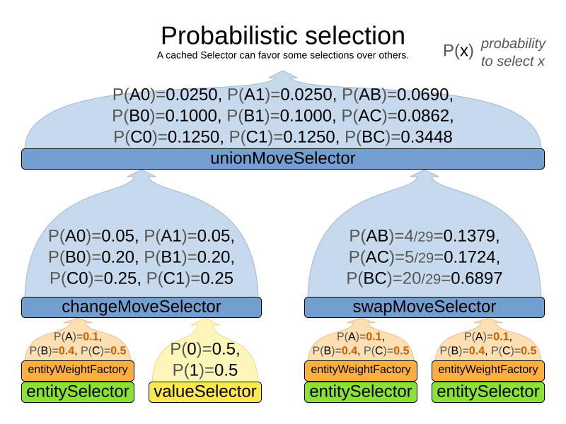
Each selection has a probabilityWeight, which determines the chance that selection will be selected:
public interface SelectionProbabilityWeightFactory<Solution_, T> {
double createProbabilityWeight(ScoreDirector<Solution_> scoreDirector, T selection);
} <entitySelector>
<cacheType>PHASE</cacheType>
<selectionOrder>PROBABILISTIC</selectionOrder>
<probabilityWeightFactoryClass>...MyEntityProbabilityWeightFactoryClass</probabilityWeightFactoryClass>
</entitySelector>For example, if there are three entities: process A (probabilityWeight 2.0), process B (probabilityWeight 0.5) and process C (probabilityWeight 0.5), then process A will be selected four times more than B and C.
|
|
10.6.7. Limited selection
Selecting all possible moves sometimes does not scale well enough, especially for construction heuristics (which don’t support acceptedCountLimit).
To limit the number of selected selection per step, apply a selectedCountLimit on the selector:
<changeMoveSelector>
<selectedCountLimit>100</selectedCountLimit>
</changeMoveSelector>|
To scale Local Search, setting acceptedCountLimit is usually better than using |
10.6.8. Mimic selection (record/replay)
During mimic selection, one normal selector records its selection and one or multiple other special selectors replay that selection. The recording selector acts as a normal selector and supports all other configuration properties. A replaying selector mimics the recording selection and supports no other configuration properties.
The recording selector needs an id.
A replaying selector must reference a recorder’s id with a mimicSelectorRef:
<cartesianProductMoveSelector>
<changeMoveSelector>
<entitySelector id="entitySelector"/>
<valueSelector variableName="period"/>
</changeMoveSelector>
<changeMoveSelector>
<entitySelector mimicSelectorRef="entitySelector"/>
<valueSelector variableName="room"/>
</changeMoveSelector>
</cartesianProductMoveSelector>Mimic selection is useful to create a composite move from two moves that affect the same entity.
10.6.9. Nearby selection
In some use cases (such as TSP and VRP, but also in non-chained variable cases), changing entities to nearby values or swapping nearby entities can heavily increase scalability and improve solution quality.
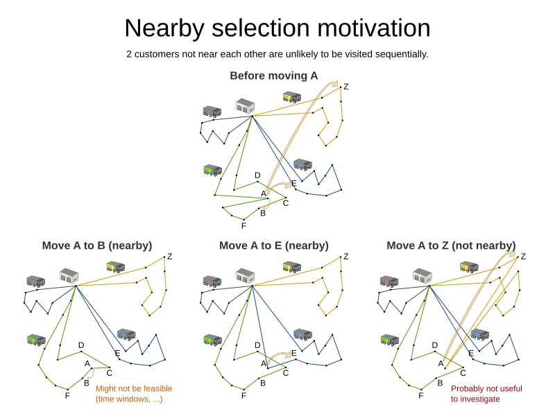
Nearby selection increases the probability of selecting an entity or value which is nearby to the first entity being moved in that move.
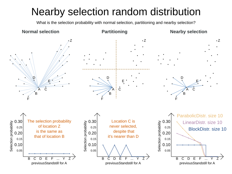
The distance between two entities or values is domain specific.
Therefore, implement the NearbyDistanceMeter interface:
public interface NearbyDistanceMeter<O, D> {
double getNearbyDistance(O origin, D destination);
}In a nutshell, when nearby selection is used in a list move selector, Origin_ is always a planning value (for example Customer) but Destination_ can be either a planning value or a planning entity. That means that in VRP the distance meter must be able to handle both Customers and Vehicles as the Destination_ destination argument:
public class CustomerNearbyDistanceMeter implements NearbyDistanceMeter<Customer, LocationAware> {
public double getNearbyDistance(Customer origin, LocationAware destination) {
return origin.getDistanceTo(destination);
}
}|
|
10.6.9.1. Nearby selection with a list variable
To configure nearby selection with a planning list variable, add a nearbySelection element in the destinationSelector, valueSelector or subListSelector
and use mimic selection to specify which destination, value, or subList should be near by the selection.
<unionMoveSelector>
<listChangeMoveSelector>
<valueSelector id="valueSelector1"/>
<destinationSelector>
<nearbySelection>
<originValueSelector mimicSelectorRef="valueSelector1"/>
<nearbyDistanceMeterClass>org.optaplanner.examples.vehiclerouting.domain.solver.nearby.CustomerNearbyDistanceMeter</nearbyDistanceMeterClass>
<parabolicDistributionSizeMaximum>40</parabolicDistributionSizeMaximum>
</nearbySelection>
</destinationSelector>
</listChangeMoveSelector>
<listSwapMoveSelector>
<valueSelector id="valueSelector2"/>
<secondaryValueSelector>
<nearbySelection>
<originValueSelector mimicSelectorRef="valueSelector2"/>
<nearbyDistanceMeterClass>org.optaplanner.examples.vehiclerouting.domain.solver.nearby.CustomerNearbyDistanceMeter</nearbyDistanceMeterClass>
<parabolicDistributionSizeMaximum>40</parabolicDistributionSizeMaximum>
</nearbySelection>
</secondaryValueSelector>
</listSwapMoveSelector>
<subListChangeMoveSelector>
<selectReversingMoveToo>true</selectReversingMoveToo>
<subListSelector id="subListSelector3"/>
<destinationSelector>
<nearbySelection>
<originSubListSelector mimicSelectorRef="subListSelector3"/>
<nearbyDistanceMeterClass>org.optaplanner.examples.vehiclerouting.domain.solver.nearby.CustomerNearbyDistanceMeter</nearbyDistanceMeterClass>
<parabolicDistributionSizeMaximum>40</parabolicDistributionSizeMaximum>
</nearbySelection>
</destinationSelector>
</subListChangeMoveSelector>
<subListSwapMoveSelector>
<selectReversingMoveToo>true</selectReversingMoveToo>
<subListSelector id="subListSelector4"/>
<secondarySubListSelector>
<nearbySelection>
<originSubListSelector mimicSelectorRef="subListSelector4"/>
<nearbyDistanceMeterClass>org.optaplanner.examples.vehiclerouting.domain.solver.nearby.CustomerNearbyDistanceMeter</nearbyDistanceMeterClass>
<parabolicDistributionSizeMaximum>40</parabolicDistributionSizeMaximum>
</nearbySelection>
</secondarySubListSelector>
</subListSwapMoveSelector>
</unionMoveSelector>10.6.9.2. Nearby selection with a chained variable
To configure nearby selection with a chained planning variable, add a nearbySelection element in the entitySelector or valueSelector
and use mimic selection to specify which entity should be near by the selection.
<unionMoveSelector>
<changeMoveSelector>
<entitySelector id="entitySelector1"/>
<valueSelector>
<nearbySelection>
<originEntitySelector mimicSelectorRef="entitySelector1"/>
<nearbyDistanceMeterClass>...CustomerNearbyDistanceMeter</nearbyDistanceMeterClass>
<parabolicDistributionSizeMaximum>40</parabolicDistributionSizeMaximum>
</nearbySelection>
</valueSelector>
</changeMoveSelector>
<swapMoveSelector>
<entitySelector id="entitySelector2"/>
<secondaryEntitySelector>
<nearbySelection>
<originEntitySelector mimicSelectorRef="entitySelector2"/>
<nearbyDistanceMeterClass>...CustomerNearbyDistanceMeter</nearbyDistanceMeterClass>
<parabolicDistributionSizeMaximum>40</parabolicDistributionSizeMaximum>
</nearbySelection>
</secondaryEntitySelector>
</swapMoveSelector>
<tailChainSwapMoveSelector>
<entitySelector id="entitySelector3"/>
<valueSelector>
<nearbySelection>
<originEntitySelector mimicSelectorRef="entitySelector3"/>
<nearbyDistanceMeterClass>...CustomerNearbyDistanceMeter</nearbyDistanceMeterClass>
<parabolicDistributionSizeMaximum>40</parabolicDistributionSizeMaximum>
</nearbySelection>
</valueSelector>
</tailChainSwapMoveSelector>
</unionMoveSelector>A distributionSizeMaximum parameter should not be 1 because if the nearest is already the planning value of the current entity, then the only move that is selectable is not doable.
To allow every element to be selected, regardless of the number of entities, only set the distribution type (so without a distributionSizeMaximum parameter):
<nearbySelection>
<nearbySelectionDistributionType>PARABOLIC_DISTRIBUTION</nearbySelectionDistributionType>
</nearbySelection>The following NearbySelectionDistributionTypes are supported:
-
BLOCK_DISTRIBUTION: Only the n nearest are selected, with an equal probability. For example, select the 20 nearest:<nearbySelection> <blockDistributionSizeMaximum>20</blockDistributionSizeMaximum> </nearbySelection> -
LINEAR_DISTRIBUTION: Nearest elements are selected with a higher probability. The probability decreases linearly.<nearbySelection> <linearDistributionSizeMaximum>40</linearDistributionSizeMaximum> </nearbySelection> -
PARABOLIC_DISTRIBUTION(recommended): Nearest elements are selected with a higher probability.<nearbySelection> <parabolicDistributionSizeMaximum>80</parabolicDistributionSizeMaximum> </nearbySelection> -
BETA_DISTRIBUTION: Selection according to a beta distribution. Slows down the solver significantly.<nearbySelection> <betaDistributionAlpha>1</betaDistributionAlpha> <betaDistributionBeta>5</betaDistributionBeta> </nearbySelection>
As always, use the Benchmarker to tweak values if desired.
10.7. Custom moves
10.7.1. Which move types might be missing in my implementation?
To determine which move types might be missing in your implementation, run a Benchmarker for a short amount of time and configure it to write the best solutions to disk. Take a look at such a best solution: it will likely be a local optima. Try to figure out if there’s a move that could get out of that local optima faster.
If you find one, implement that coarse-grained move, mix it with the existing moves and benchmark it against the previous configurations to see if you want to keep it.
10.7.2. Custom moves introduction
Instead of using the generic Moves (such as ChangeMove) you can also implement your own Move.
Generic and custom MoveSelectors can be combined as desired.
A custom Move can be tailored to work to the advantage of your constraints.
For example in examination scheduling, changing the period of an exam A
would also change the period of all the other exams that need to coincide with exam A.
A custom Move is far more work to implement and much harder to avoid bugs than a generic Move.
After implementing a custom Move, turn on environmentMode FULL_ASSERT to check for score corruptions.
10.7.3. The Move interface
All moves implement the Move interface:
public interface Move<Solution_> {
boolean isMoveDoable(ScoreDirector<Solution_> scoreDirector);
Move<Solution_> doMove(ScoreDirector<Solution_> scoreDirector);
...
}To implement a custom move, it’s recommended to extend AbstractMove instead implementing Move directly.
OptaPlanner calls AbstractMove.doMove(ScoreDirector), which calls doMoveOnGenuineVariables(ScoreDirector).
For example in cloud balancing, this move changes one process to another computer:
public class CloudComputerChangeMove extends AbstractMove<CloudBalance> {
private CloudProcess cloudProcess;
private CloudComputer toCloudComputer;
public CloudComputerChangeMove(CloudProcess cloudProcess, CloudComputer toCloudComputer) {
this.cloudProcess = cloudProcess;
this.toCloudComputer = toCloudComputer;
}
@Override
protected void doMoveOnGenuineVariables(ScoreDirector<CloudBalance> scoreDirector) {
scoreDirector.beforeVariableChanged(cloudProcess, "computer");
cloudProcess.setComputer(toCloudComputer);
scoreDirector.afterVariableChanged(cloudProcess, "computer");
}
// ...
}The implementation must notify the ScoreDirector of any changes it makes to planning entity’s variables:
Call the scoreDirector.beforeVariableChanged(Object, String) and scoreDirector.afterVariableChanged(Object, String)
methods directly before and after modifying an entity’s planning variable.
The example move above is a fine-grained move because it changes only one planning variable. On the other hand, a coarse-grained move changes multiple entities or multiple planning variables in a single move, usually to avoid breaking hard constraints by making multiple related changes at once. For example, a swap move is really just two change moves, but it keeps those two changes together.
|
A |
OptaPlanner automatically filters out non doable moves by calling the isMoveDoable(ScoreDirector) method on each selected move.
A non doable move is:
-
A move that changes nothing on the current solution. For example, moving process
P1on computerXto computerXis not doable, because it is already there. -
A move that is impossible to do on the current solution. For example, moving process
P1to computerQ(whenQisn’t in the list of computers) is not doable because it would assign a planning value that’s not inside the planning variable’s value range.
In the cloud balancing example, a move which assigns a process to the computer it’s already assigned to is not doable:
@Override
public boolean isMoveDoable(ScoreDirector<CloudBalance> scoreDirector) {
return !Objects.equals(cloudProcess.getComputer(), toCloudComputer);
}We don’t need to check if toCloudComputer is in the value range,
because we only generate moves for which that is the case.
A move that is currently not doable can become doable when the working solution changes in a later step,
otherwise we probably shouldn’t have created it in the first place.
Each move has an undo move: a move (normally of the same type) which does the exact opposite.
In the cloud balancing example the undo move of P1 {X → Y} is the move P1 {Y → X}.
The undo move of a move is created when the Move is being done on the current solution,
before the genuine variables change:
@Override
public CloudComputerChangeMove createUndoMove(ScoreDirector<CloudBalance> scoreDirector) {
return new CloudComputerChangeMove(cloudProcess, cloudProcess.getComputer());
}Notice that if P1 would have already been moved to Y, the undo move would create the move P1 {Y → Y},
instead of the move P1 {Y → X}.
A solver phase might do and undo the same Move more than once.
In fact, many solver phases will iteratively do and undo a number of moves to evaluate them,
before selecting one of those and doing that move again (without undoing it the last time).
Always implement the toString() method to keep OptaPlanner’s logs readable.
Keep it non-verbose and make it consistent with the generic moves:
public String toString() {
return cloudProcess + " {" + cloudProcess.getComputer() + " -> " + toCloudComputer + "}";
}Optionally, implement the getSimpleMoveTypeDescription() method to support
picked move statistics:
@Override
public String getSimpleMoveTypeDescription() {
return "CloudComputerChangeMove(CloudProcess.computer)";
}10.7.3.1. Custom move: rebase()
For multithreaded incremental solving,
the custom move must implement the rebase() method:
@Override
public CloudComputerChangeMove rebase(ScoreDirector<CloudBalance> destinationScoreDirector) {
return new CloudComputerChangeMove(destinationScoreDirector.lookUpWorkingObject(cloudProcess),
destinationScoreDirector.lookUpWorkingObject(toCloudComputer));
}Rebasing a move takes a move generated of one working solution and creates a new move that does the same change as the original move, but rewired as if was generated off of the destination working solution. This allows multithreaded solving to migrate moves from one thread to another.
The lookUpWorkingObject() method translates a planning entity instance or problem fact instance
from one working solution to that of the destination’s working solution.
Internally it often uses a mapping technique based on the planning ID.
To rebase lists or arrays in bulk, use rebaseList() and rebaseArray() on AbstractMove.
10.7.3.2. Custom move: getPlanningEntities() and getPlanningValues()
A custom move should also implement the getPlanningEntities() and getPlanningValues() methods.
Those are used by entity tabu and value tabu respectively.
They are called after the Move has already been done.
@Override
public Collection<? extends Object> getPlanningEntities() {
return Collections.singletonList(cloudProcess);
}
@Override
public Collection<? extends Object> getPlanningValues() {
return Collections.singletonList(toCloudComputer);
}If the Move changes multiple planning entities, such as in a swap move,
return all of them in getPlanningEntities()
and return all their values (to which they are changing) in getPlanningValues().
@Override
public Collection<? extends Object> getPlanningEntities() {
return Arrays.asList(leftCloudProcess, rightCloudProcess);
}
@Override
public Collection<? extends Object> getPlanningValues() {
return Arrays.asList(leftCloudProcess.getComputer(), rightCloudProcess.getComputer());
}10.7.3.3. Custom move: equals() and hashCode()
A Move must implement the equals() and hashCode() methods for move tabu.
Two moves which make the same change on a solution, should be equal ideally.
@Override
public boolean equals(Object o) {
if (this == o) {
return true;
} else if (o instanceof CloudComputerChangeMove) {
CloudComputerChangeMove other = (CloudComputerChangeMove) o;
return new EqualsBuilder()
.append(cloudProcess, other.cloudProcess)
.append(toCloudComputer, other.toCloudComputer)
.isEquals();
} else {
return false;
}
}
@Override
public int hashCode() {
return new HashCodeBuilder()
.append(cloudProcess)
.append(toCloudComputer)
.toHashCode();
}Notice that it checks if the other move is an instance of the same move type.
This instanceof check is important because a move are compared to a move of another move type.
For example a ChangeMove and SwapMove are compared.
10.7.4. Generating custom moves
Now, let’s generate instances of this custom Move class.
There are 2 ways:
10.7.4.1. MoveListFactory: the easy way to generate custom moves
The easiest way to generate custom moves is by implementing the interface MoveListFactory:
public interface MoveListFactory<Solution_> {
List<Move> createMoveList(Solution_ solution);
}For example:
public class CloudComputerChangeMoveFactory implements MoveListFactory<CloudBalance> {
@Override
public List<CloudComputerChangeMove> createMoveList(CloudBalance cloudBalance) {
List<CloudComputerChangeMove> moveList = new ArrayList<>();
List<CloudComputer> cloudComputerList = cloudBalance.getComputerList();
for (CloudProcess cloudProcess : cloudBalance.getProcessList()) {
for (CloudComputer cloudComputer : cloudComputerList) {
moveList.add(new CloudComputerChangeMove(cloudProcess, cloudComputer));
}
}
return moveList;
}
}Simple configuration (which can be nested in a unionMoveSelector just like any other MoveSelector):
<moveListFactory>
<moveListFactoryClass>org.optaplanner.examples.cloudbalancing.optional.solver.move.CloudComputerChangeMoveFactory</moveListFactoryClass>
</moveListFactory>Advanced configuration:
<moveListFactory>
... <!-- Normal moveSelector properties -->
<moveListFactoryClass>org.optaplanner.examples.cloudbalancing.optional.solver.move.CloudComputerChangeMoveFactory</moveListFactoryClass>
<moveListFactoryCustomProperties>
...<!-- Custom properties -->
</moveListFactoryCustomProperties>
</moveListFactory>Because the MoveListFactory generates all moves at once in a List<Move>,
it does not support cacheType JUST_IN_TIME.
Therefore, moveListFactory uses cacheType STEP by default and it scales badly.
To configure values of a MoveListFactory dynamically in the solver configuration
(so the Benchmarker can tweak those parameters),
add the moveListFactoryCustomProperties element and use custom properties.
|
A custom |
10.7.4.2. MoveIteratorFactory: generate Custom moves just in time
Use this advanced form to generate custom moves Just In Time
by implementing the MoveIteratorFactory interface:
public interface MoveIteratorFactory<Solution_> {
long getSize(ScoreDirector<Solution_> scoreDirector);
Iterator<Move> createOriginalMoveIterator(ScoreDirector<Solution_> scoreDirector);
Iterator<Move> createRandomMoveIterator(ScoreDirector<Solution_> scoreDirector, Random workingRandom);
}The getSize() method must return an estimation of the size.
It doesn’t need to be correct, but it’s better too big than too small.
The createOriginalMoveIterator method is called if the selectionOrder is ORIGINAL or if it is cached.
The createRandomMoveIterator method is called for selectionOrder RANDOM combined with cacheType JUST_IN_TIME.
|
Don’t create a collection (array, list, set or map) of |
Simple configuration (which can be nested in a unionMoveSelector just like any other MoveSelector):
<moveIteratorFactory>
<moveIteratorFactoryClass>...</moveIteratorFactoryClass>
</moveIteratorFactory>Advanced configuration:
<moveIteratorFactory>
... <!-- Normal moveSelector properties -->
<moveIteratorFactoryClass>...</moveIteratorFactoryClass>
<moveIteratorFactoryCustomProperties>
...<!-- Custom properties -->
</moveIteratorFactoryCustomProperties>
</moveIteratorFactory>To configure values of a MoveIteratorFactory dynamically in the solver configuration
(so the Benchmarker can tweak those parameters),
add the moveIteratorFactoryCustomProperties element and use custom properties.
|
A custom |
11. Exhaustive search
11.1. Overview
Exhaustive Search will always find the global optimum and recognize it too. That being said, it doesn’t scale (not even beyond toy data sets) and is therefore mostly useless.
11.2. Brute force
11.2.1. Algorithm description
The Brute Force algorithm creates and evaluates every possible solution.
Notice that it creates a search tree that explodes exponentially as the problem size increases, so it hits a scalability wall.
|
Brute Force is mostly unusable for a real-world problem due to time limitations, as shown in scalability of Exhaustive Search. |
11.2.2. Configuration
Simplest configuration of Brute Force:
<solver xmlns="https://www.optaplanner.org/xsd/solver" xmlns:xsi="http://www.w3.org/2001/XMLSchema-instance"
xsi:schemaLocation="https://www.optaplanner.org/xsd/solver https://www.optaplanner.org/xsd/solver/solver.xsd">
...
<exhaustiveSearch>
<exhaustiveSearchType>BRUTE_FORCE</exhaustiveSearchType>
</exhaustiveSearch>
</solver>11.3. Branch and bound
11.3.1. Algorithm description
Branch And Bound also explores nodes in an exponential search tree, but it investigates more promising nodes first and prunes away worthless nodes.
For each node, Branch And Bound calculates the optimistic bound: the best possible score to which that node can lead to. If the optimistic bound of a node is lower or equal to the global pessimistic bound, then it prunes away that node (including the entire branch of all its subnodes).
|
Academic papers use the term lower bound instead of optimistic bound (and the term upper bound instead of pessimistic bound), because they minimize the score. OptaPlanner maximizes the score (because it supports combining negative and positive constraints). Therefore, for clarity, it uses different terms, as it would be confusing to use the term lower bound for a bound which is always higher. |
For example: at index 14, it sets the global pessimistic bound to -2.
Because all solutions reachable from the node visited at index 11 will have a score lower or equal to -2 (the node’s optimistic bound), they can be pruned away.
Notice that Branch And Bound (much like Brute Force) creates a search tree that explodes exponentially as the problem size increases. So it hits the same scalability wall, only a little bit later.
|
Branch And Bound is mostly unusable for a real-world problem due to time limitations, as shown in scalability of Exhaustive Search. |
11.3.2. Configuration
Simplest configuration of Branch And Bound:
<solver xmlns="https://www.optaplanner.org/xsd/solver" xmlns:xsi="http://www.w3.org/2001/XMLSchema-instance"
xsi:schemaLocation="https://www.optaplanner.org/xsd/solver https://www.optaplanner.org/xsd/solver/solver.xsd">
...
<exhaustiveSearch>
<exhaustiveSearchType>BRANCH_AND_BOUND</exhaustiveSearchType>
</exhaustiveSearch>
</solver>|
For the pruning to work with the default |
Advanced configuration:
<exhaustiveSearch>
<exhaustiveSearchType>BRANCH_AND_BOUND</exhaustiveSearchType>
<nodeExplorationType>DEPTH_FIRST</nodeExplorationType>
<entitySorterManner>DECREASING_DIFFICULTY_IF_AVAILABLE</entitySorterManner>
<valueSorterManner>INCREASING_STRENGTH_IF_AVAILABLE</valueSorterManner>
</exhaustiveSearch>The nodeExplorationType options are:
-
DEPTH_FIRST(default): Explore deeper nodes first (and then a better score and then a better optimistic bound). Deeper nodes (especially leaf nodes) often improve the pessimistic bound. A better pessimistic bound allows pruning more nodes to reduce the search space.<exhaustiveSearch> <exhaustiveSearchType>BRANCH_AND_BOUND</exhaustiveSearchType> <nodeExplorationType>DEPTH_FIRST</nodeExplorationType> </exhaustiveSearch> -
BREADTH_FIRST(not recommended): Explore nodes layer by layer (and then a better score and then a better optimistic bound). Scales terribly in memory (and usually in performance too).<exhaustiveSearch> <exhaustiveSearchType>BRANCH_AND_BOUND</exhaustiveSearchType> <nodeExplorationType>BREADTH_FIRST</nodeExplorationType> </exhaustiveSearch> -
SCORE_FIRST: Explore nodes with a better score first (and then a better optimistic bound and then deeper nodes first). Might scale as terribly asBREADTH_FIRSTin some cases.<exhaustiveSearch> <exhaustiveSearchType>BRANCH_AND_BOUND</exhaustiveSearchType> <nodeExplorationType>SCORE_FIRST</nodeExplorationType> </exhaustiveSearch> -
OPTIMISTIC_BOUND_FIRST: Explore nodes with a better optimistic bound first (and then a better score and then deeper nodes first). Might scale as terribly asBREADTH_FIRSTin some cases.<exhaustiveSearch> <exhaustiveSearchType>BRANCH_AND_BOUND</exhaustiveSearchType> <nodeExplorationType>OPTIMISTIC_BOUND_FIRST</nodeExplorationType> </exhaustiveSearch>
The entitySorterManner options are:
-
DECREASING_DIFFICULTY: Initialize the more difficult planning entities first. This usually increases pruning (and therefore improves scalability). Requires the model to support planning entity difficulty comparison. -
DECREASING_DIFFICULTY_IF_AVAILABLE(default): If the model supports planning entity difficulty comparison, behave likeDECREASING_DIFFICULTY, else likeNONE. -
NONE: Initialize the planning entities in original order.
The valueSorterManner options are:
-
INCREASING_STRENGTH: Evaluate the planning values in increasing strength. Requires the model to support planning value strength comparison. -
INCREASING_STRENGTH_IF_AVAILABLE(default): If the model supports planning value strength comparison, behave likeINCREASING_STRENGTH, else likeNONE. -
DECREASING_STRENGTH: Evaluate the planning values in decreasing strength. Requires the model to support planning value strength comparison. -
DECREASING_STRENGTH_IF_AVAILABLE: If the model supports planning value strength comparison, behave likeDECREASING_STRENGTH, else likeNONE. -
NONE: Try the planning values in original order.
11.4. Scalability of exhaustive search
Exhaustive Search variants suffer from two big scalability issues:
-
They scale terribly memory wise.
-
They scale horribly performance wise.
As shown in these time spent graphs from the Benchmarker, Brute Force and Branch And Bound both hit a performance scalability wall. For example, on N queens it hits wall at a few dozen queens:
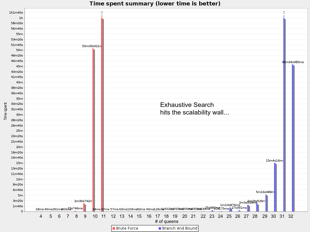
In most use cases, such as Cloud Balancing, the wall appears out of thin air:
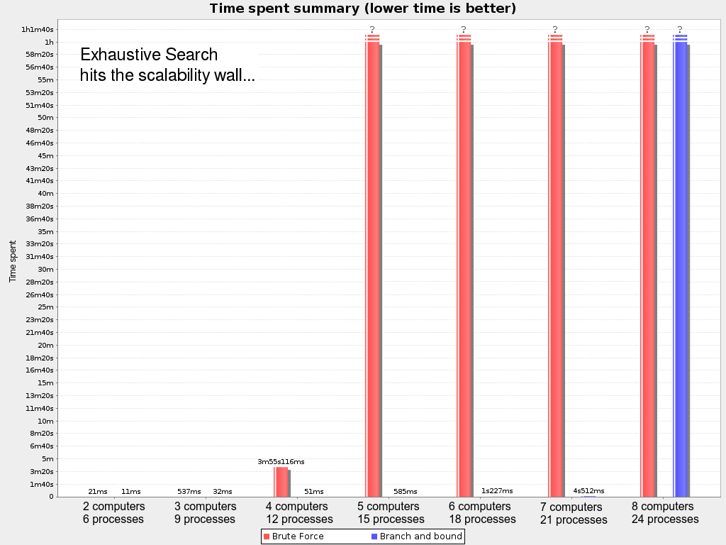
Exhaustive Search hits this wall on small datasets already, so in production these optimizations algorithms are mostly useless. Use Construction Heuristics with Local Search instead: those can handle thousands of queens/computers easily.
|
Throwing hardware at these scalability issues has no noticeable impact. Newer and more hardware are just a drop in the ocean. Moore’s law cannot win against the onslaught of a few more planning entities in the dataset. |
12. Construction heuristics
12.1. Overview
A construction heuristic builds a pretty good initial solution in a finite length of time. Its solution isn’t always feasible, but it finds it fast so metaheuristics can finish the job.
Construction heuristics terminate automatically, so there’s usually no need to configure a Termination on the construction heuristic phase specifically.
12.2. First fit
12.2.1. Algorithm description
The First Fit algorithm cycles through all the planning entities (in default order), initializing one planning entity at a time. It assigns the planning entity to the best available planning value, taking the already initialized planning entities into account. It terminates when all planning entities have been initialized. It never changes a planning entity after it has been assigned.
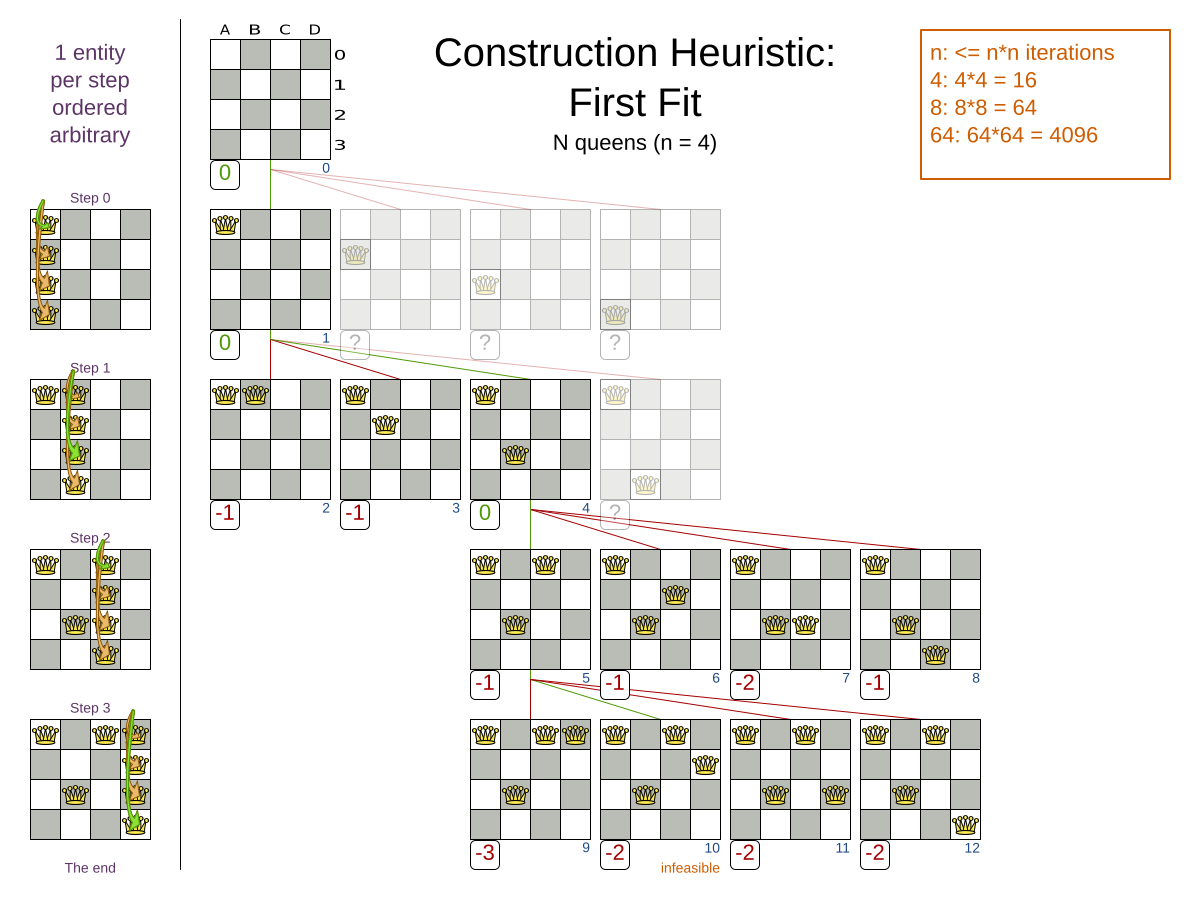
Notice that it starts with putting Queen A into row 0 (and never moving it later), which makes it impossible to reach the optimal solution.
Suffixing this construction heuristic with metaheuristics can remedy that.
12.2.2. Configuration
Simple configuration:
<constructionHeuristic>
<constructionHeuristicType>FIRST_FIT</constructionHeuristicType>
</constructionHeuristic>Advanced configuration:
<constructionHeuristic>
<constructionHeuristicType>FIRST_FIT</constructionHeuristicType>
<...MoveSelector/>
<...MoveSelector/>
...
</constructionHeuristic>For scaling out, see scaling construction heuristics. For a very advanced configuration, see Allocate Entity From Queue.
12.3. First fit decreasing
12.3.1. Algorithm description
Like First Fit, but assigns the more difficult planning entities first, because they are less likely to fit in the leftovers. So it sorts the planning entities on decreasing difficulty.
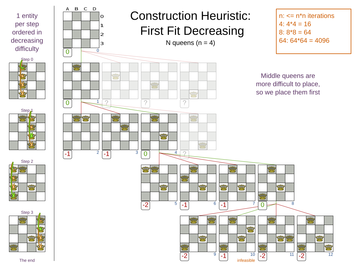
Requires the model to support planning entity difficulty comparison.
|
One would expect that this algorithm has better results than First Fit. That’s usually the case, but not always. |
12.3.2. Configuration
Simple configuration:
<constructionHeuristic>
<constructionHeuristicType>FIRST_FIT_DECREASING</constructionHeuristicType>
</constructionHeuristic>Advanced configuration:
<constructionHeuristic>
<constructionHeuristicType>FIRST_FIT_DECREASING</constructionHeuristicType>
<...MoveSelector/>
<...MoveSelector/>
...
</constructionHeuristic>For scaling out, see scaling construction heuristics. For a very advanced configuration, see Allocate Entity From Queue.
12.4. Weakest fit
12.4.1. Algorithm description
Like First Fit, but uses the weaker planning values first, because the strong planning values are more likely to be able to accommodate later planning entities. So it sorts the planning values on increasing strength.
Requires the model to support planning value strength comparison.
|
Do not presume that this algorithm has better results than First Fit. That’s often not the case. |
12.4.2. Configuration
Simple configuration:
<constructionHeuristic>
<constructionHeuristicType>WEAKEST_FIT</constructionHeuristicType>
</constructionHeuristic>Advanced configuration:
<constructionHeuristic>
<constructionHeuristicType>WEAKEST_FIT</constructionHeuristicType>
<...MoveSelector/>
<...MoveSelector/>
...
</constructionHeuristic>For scaling out, see scaling construction heuristics. For a very advanced configuration, see Allocate Entity From Queue.
12.5. Weakest fit decreasing
12.5.1. Algorithm description
Combines First Fit Decreasing and Weakest Fit. So it sorts the planning entities on decreasing difficulty and the planning values on increasing strength.
Requires the model to support planning entity difficulty comparison and planning value strength comparison.
|
Do not presume that this algorithm has better results than First Fit Decreasing. That’s often not the case. However, it is usually better than Weakest Fit. |
12.5.2. Configuration
Simple configuration:
<constructionHeuristic>
<constructionHeuristicType>WEAKEST_FIT_DECREASING</constructionHeuristicType>
</constructionHeuristic>Advanced configuration:
<constructionHeuristic>
<constructionHeuristicType>WEAKEST_FIT_DECREASING</constructionHeuristicType>
<...MoveSelector/>
<...MoveSelector/>
...
</constructionHeuristic>For scaling out, see scaling construction heuristics. For a very advanced configuration, see Allocate Entity From Queue.
12.6. Strongest fit
12.6.1. Algorithm description
Like First Fit, but uses the strong planning values first, because the strong planning values are more likely to have a lower soft cost to use. So it sorts the planning values on decreasing strength.
Requires the model to support planning value strength comparison.
|
Do not presume that this algorithm has better results than First Fit or Weakest Fit. That’s often not the case. |
12.6.2. Configuration
Simple configuration:
<constructionHeuristic>
<constructionHeuristicType>STRONGEST_FIT</constructionHeuristicType>
</constructionHeuristic>Advanced configuration:
<constructionHeuristic>
<constructionHeuristicType>STRONGEST_FIT</constructionHeuristicType>
<...MoveSelector/>
<...MoveSelector/>
...
</constructionHeuristic>For scaling out, see scaling construction heuristics. For a very advanced configuration, see Allocate Entity From Queue.
12.7. Strongest fit decreasing
12.7.1. Algorithm description
Combines First Fit Decreasing and Strongest Fit. So it sorts the planning entities on decreasing difficulty and the planning values on decreasing strength.
Requires the model to support planning entity difficulty comparison and planning value strength comparison.
|
Do not presume that this algorithm has better results than First Fit Decreasing or Weakest Fit Decreasing. That’s often not the case. However, it is usually better than Strongest Fit. |
12.7.2. Configuration
Simple configuration:
<constructionHeuristic>
<constructionHeuristicType>STRONGEST_FIT_DECREASING</constructionHeuristicType>
</constructionHeuristic>Advanced configuration:
<constructionHeuristic>
<constructionHeuristicType>STRONGEST_FIT_DECREASING</constructionHeuristicType>
<...MoveSelector/>
<...MoveSelector/>
...
</constructionHeuristic>For scaling out, see scaling construction heuristics. For a very advanced configuration, see Allocate Entity From Queue.
12.8. Allocate entity from queue
12.8.1. Algorithm description
Allocate Entity From Queue is a versatile, generic form of First Fit, First Fit Decreasing, Weakest Fit, Weakest Fit Decreasing, Strongest Fit and Strongest Fit Decreasing. It works like this:
-
Put all entities in a queue.
-
Assign the first entity (from that queue) to the best value.
-
Repeat until all entities are assigned.
12.8.2. Configuration
Simple configuration:
<constructionHeuristic>
<constructionHeuristicType>ALLOCATE_ENTITY_FROM_QUEUE</constructionHeuristicType>
</constructionHeuristic>Verbose simple configuration:
<constructionHeuristic>
<constructionHeuristicType>ALLOCATE_ENTITY_FROM_QUEUE</constructionHeuristicType>
<entitySorterManner>DECREASING_DIFFICULTY_IF_AVAILABLE</entitySorterManner>
<valueSorterManner>INCREASING_STRENGTH_IF_AVAILABLE</valueSorterManner>
</constructionHeuristic>The entitySorterManner options are:
-
DECREASING_DIFFICULTY: Initialize the more difficult planning entities first. This usually increases pruning (and therefore improves scalability). Requires the model to support planning entity difficulty comparison. -
DECREASING_DIFFICULTY_IF_AVAILABLE(default): If the model supports planning entity difficulty comparison, behave likeDECREASING_DIFFICULTY, else likeNONE. -
NONE: Initialize the planning entities in original order.
The valueSorterManner options are:
-
INCREASING_STRENGTH: Evaluate the planning values in increasing strength. Requires the model to support planning value strength comparison. -
INCREASING_STRENGTH_IF_AVAILABLE(default): If the model supports planning value strength comparison, behave likeINCREASING_STRENGTH, else likeNONE. -
DECREASING_STRENGTH: Evaluate the planning values in decreasing strength. Requires the model to support planning value strength comparison. -
DECREASING_STRENGTH_IF_AVAILABLE: If the model supports planning value strength comparison, behave likeDECREASING_STRENGTH, else likeNONE. -
NONE: Try the planning values in original order.
Advanced configuration with Weakest Fit Decreasing for a single entity class with one variable:
<constructionHeuristic>
<queuedEntityPlacer>
<entitySelector id="placerEntitySelector">
<cacheType>PHASE</cacheType>
<selectionOrder>SORTED</selectionOrder>
<sorterManner>DECREASING_DIFFICULTY</sorterManner>
</entitySelector>
<changeMoveSelector>
<entitySelector mimicSelectorRef="placerEntitySelector"/>
<valueSelector>
<cacheType>PHASE</cacheType>
<selectionOrder>SORTED</selectionOrder>
<sorterManner>INCREASING_STRENGTH</sorterManner>
</valueSelector>
</changeMoveSelector>
</queuedEntityPlacer>
</constructionHeuristic>Per step, the QueuedEntityPlacer selects one uninitialized entity from the EntitySelector
and applies the winning Move (out of all the moves for that entity generated by the MoveSelector).
The mimic selection ensures that the winning Move changes only the selected entity.
To customize the entity or value sorting, see sorted selection. For scaling out, see scaling construction heuristics.
If there are multiple planning variables, there’s one ChangeMoveSelector per planning variable,
which are either in a cartesian product or in sequential steps,
similar to the less verbose configuration.
12.8.3. Multiple entity classes
The easiest way to deal with multiple entity classes is to run a separate Construction Heuristic for each entity class:
<constructionHeuristic>
<queuedEntityPlacer>
<entitySelector id="placerEntitySelector">
<entityClass>...DogEntity</entityClass>
<cacheType>PHASE</cacheType>
</entitySelector>
<changeMoveSelector>
<entitySelector mimicSelectorRef="placerEntitySelector"/>
</changeMoveSelector>
</queuedEntityPlacer>
...
</constructionHeuristic>
<constructionHeuristic>
<queuedEntityPlacer>
<entitySelector id="placerEntitySelector">
<entityClass>...CatEntity</entityClass>
<cacheType>PHASE</cacheType>
</entitySelector>
<changeMoveSelector>
<entitySelector mimicSelectorRef="placerEntitySelector"/>
</changeMoveSelector>
</queuedEntityPlacer>
...
</constructionHeuristic>12.8.4. Pick early type
There are several pick early types for Construction Heuristics:
-
NEVER: Evaluate all the selected moves to initialize the variable(s). This is the default if the InitializingScoreTrend is notONLY_DOWN.<constructionHeuristic> ... <forager> <pickEarlyType>NEVER</pickEarlyType> </forager> </constructionHeuristic> -
FIRST_NON_DETERIORATING_SCORE: Initialize the variable(s) with the first move that doesn’t deteriorate the score, ignore the remaining selected moves. This is the default if the InitializingScoreTrend isONLY_DOWN.<constructionHeuristic> ... <forager> <pickEarlyType>FIRST_NON_DETERIORATING_SCORE</pickEarlyType> </forager> </constructionHeuristic>If there are only negative constraints, but the InitializingScoreTrend is strictly not
ONLY_DOWN, it can sometimes make sense to apply FIRST_NON_DETERIORATING_SCORE. Use the Benchmarker to decide if the score quality loss is worth the time gain. -
FIRST_FEASIBLE_SCORE: Initialize the variable(s) with the first move that has a feasible score.<constructionHeuristic> ... <forager> <pickEarlyType>FIRST_FEASIBLE_SCORE</pickEarlyType> </forager> </constructionHeuristic>If the InitializingScoreTrend is
ONLY_DOWN, useFIRST_FEASIBLE_SCORE_OR_NON_DETERIORATING_HARDinstead, because that’s faster without any disadvantages. -
FIRST_FEASIBLE_SCORE_OR_NON_DETERIORATING_HARD: Initialize the variable(s) with the first move that doesn’t deteriorate the feasibility of the score any further.<constructionHeuristic> ... <forager> <pickEarlyType>FIRST_FEASIBLE_SCORE_OR_NON_DETERIORATING_HARD</pickEarlyType> </forager> </constructionHeuristic>
12.9. Allocate to value from queue
12.9.1. Algorithm description
Allocate To Value From Queue works like this:
-
Put all values in a round-robin queue.
-
Assign the best entity to the first value (from that queue).
-
Repeat until all entities are assigned.
12.9.2. Configuration
Simple configuration:
<constructionHeuristic>
<constructionHeuristicType>ALLOCATE_TO_VALUE_FROM_QUEUE</constructionHeuristicType>
</constructionHeuristic>Verbose simple configuration:
<constructionHeuristic>
<constructionHeuristicType>ALLOCATE_TO_VALUE_FROM_QUEUE</constructionHeuristicType>
<entitySorterManner>DECREASING_DIFFICULTY_IF_AVAILABLE</entitySorterManner>
<valueSorterManner>INCREASING_STRENGTH_IF_AVAILABLE</valueSorterManner>
</constructionHeuristic>Advanced configuration for a single entity class with a single variable:
<constructionHeuristic>
<queuedValuePlacer>
<valueSelector id="placerValueSelector">
<cacheType>PHASE</cacheType>
<selectionOrder>SORTED</selectionOrder>
<sorterManner>INCREASING_STRENGTH</sorterManner>
</valueSelector>
<changeMoveSelector>
<entitySelector>
<cacheType>PHASE</cacheType>
<selectionOrder>SORTED</selectionOrder>
<sorterManner>DECREASING_DIFFICULTY</sorterManner>
</entitySelector>
<valueSelector mimicSelectorRef="placerValueSelector"/>
</changeMoveSelector>
</queuedValuePlacer>
</constructionHeuristic>For scaling out, see scaling construction heuristics.
12.10. Cheapest insertion
12.10.1. Algorithm description
The Cheapest Insertion algorithm cycles through all the planning values for all the planning entities, initializing one planning entity at a time. It assigns a planning entity to the best available planning value (out of all the planning entities and values), taking the already initialized planning entities into account. It terminates when all planning entities have been initialized. It never changes a planning entity after it has been assigned.
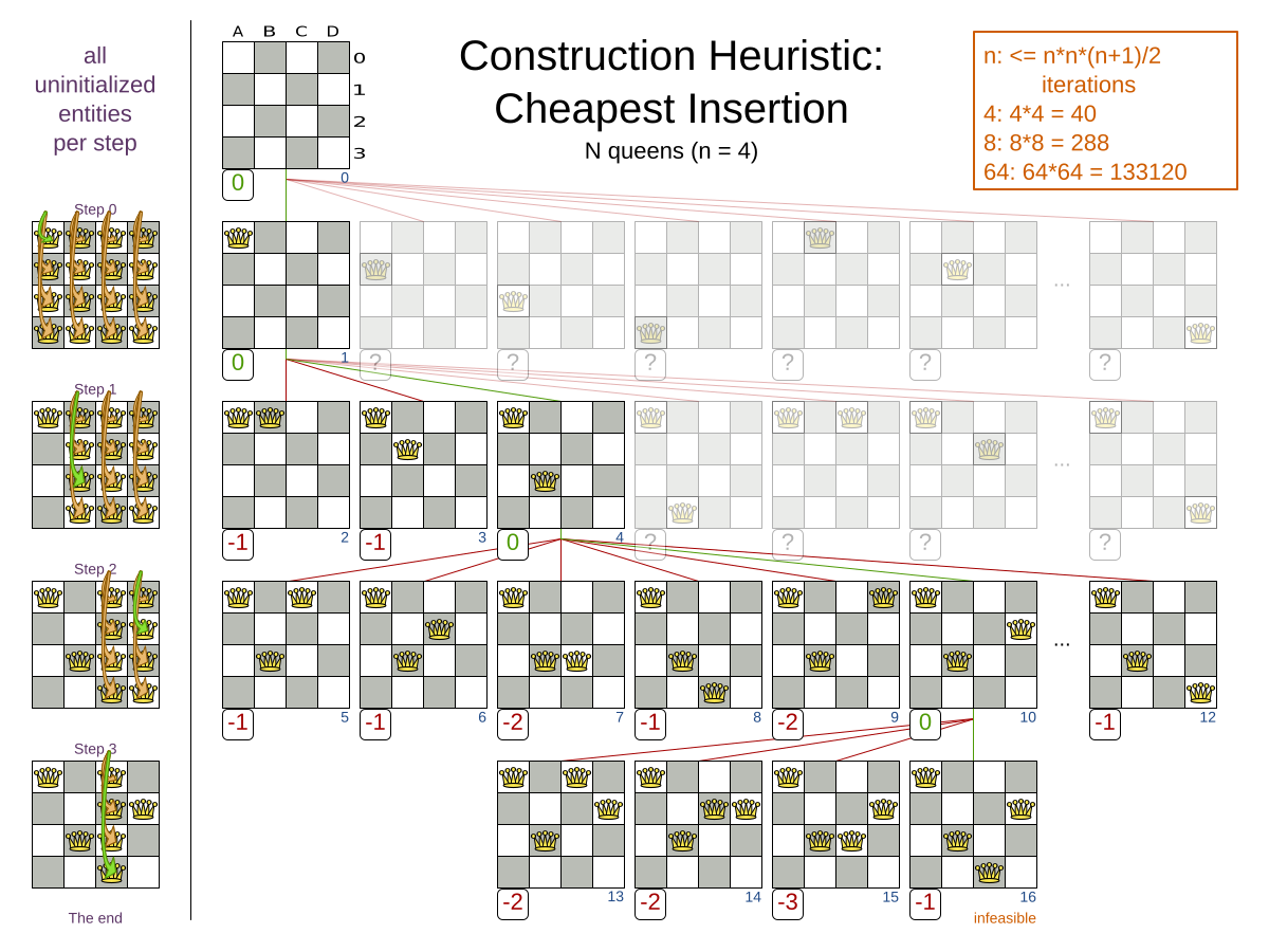
|
Cheapest Insertion scales considerably worse than First Fit, etc. |
12.10.2. Configuration
Simple configuration:
<constructionHeuristic>
<constructionHeuristicType>CHEAPEST_INSERTION</constructionHeuristicType>
</constructionHeuristic>Advanced configuration:
<constructionHeuristic>
<constructionHeuristicType>CHEAPEST_INSERTION</constructionHeuristicType>
<...MoveSelector/>
<...MoveSelector/>
...
</constructionHeuristic>For scaling out, see scaling construction heuristics. For a very advanced configuration, see Allocate from pool.
12.11. Regret insertion
12.11.1. Algorithm description
The Regret Insertion algorithm behaves like the Cheapest Insertion algorithm. It also cycles through all the planning values for all the planning entities, initializing one planning entity at a time. But instead of picking the entity-value combination with the best score, it picks the entity which has the largest score loss between its best and second best value assignment. It then assigns that entity to its best value, to avoid regretting not having done that.
12.11.2. Configuration
This algorithm has not been implemented yet.
12.12. Allocate from pool
12.12.1. Algorithm description
Allocate From Pool is a versatile, generic form of Cheapest Insertion and Regret Insertion. It works like this:
-
Put all entity-value combinations in a pool.
-
Assign the best entity to best value.
-
Repeat until all entities are assigned.
12.12.2. Configuration
Simple configuration:
<constructionHeuristic>
<constructionHeuristicType>ALLOCATE_FROM_POOL</constructionHeuristicType>
</constructionHeuristic>Verbose simple configuration:
<constructionHeuristic>
<constructionHeuristicType>ALLOCATE_FROM_POOL</constructionHeuristicType>
<entitySorterManner>DECREASING_DIFFICULTY_IF_AVAILABLE</entitySorterManner>
<valueSorterManner>INCREASING_STRENGTH_IF_AVAILABLE</valueSorterManner>
</constructionHeuristic>The entitySorterManner and valueSorterManner options are described in Allocate Entity From Queue.
Advanced configuration with Cheapest Insertion for a single entity class with a single variable:
<constructionHeuristic>
<pooledEntityPlacer>
<changeMoveSelector>
<entitySelector id="placerEntitySelector">
<cacheType>PHASE</cacheType>
<selectionOrder>SORTED</selectionOrder>
<sorterManner>DECREASING_DIFFICULTY</sorterManner>
</entitySelector>
<valueSelector>
<cacheType>PHASE</cacheType>
<selectionOrder>SORTED</selectionOrder>
<sorterManner>INCREASING_STRENGTH</sorterManner>
</valueSelector>
</changeMoveSelector>
</pooledEntityPlacer>
</constructionHeuristic>Per step, the PooledEntityPlacer applies the winning Move (out of all the moves for that entity generated by the MoveSelector).
To customize the entity or value sorting, see sorted selection.
Other Selector customization (such as filtering and limiting) is supported too.
For scaling out, see scaling construction heuristics.
12.13. Scaling construction heuristics
If the Construction Heuristic takes a long time to solve and create an initial solution, there is too little time left for Local Search to reach a near optimal solution.
Ideally, a Construction Heuristic should take less than 20 seconds from scratch and less than 50 milliseconds in real-time planning, so there is plenty of time left for Local Search. If the Benchmarker proves that this is not the case, there’s a number of improvements that can be done:
12.13.1. InitializingScoreTrend shortcuts
If the InitializingScoreTrend is ONLY_DOWN, a Construction Heuristic algorithm (such as First Fit) is faster:
for an entity, it picks the first move for which the score does not deteriorate the last step score, ignoring all subsequent moves in that step.
It can take that shortcut without reducing solution quality, because a down trend guarantees that initializing any additional planning variable can only make the score the same or worse. So if a move has the same score as before the planning variable was initialized, then no other move can have a better score.
12.13.2. Scaling multiple planning variables in construction heuristics
There are two ways to deal with multiple planning variables,
depending on how their ChangeMoves are combined:
-
Cartesian product (default): All variables of the selected entity are assigned together. This usually results in a better solution quality, but it scales poorly because it tries every combination of variables. For example:
<constructionHeuristic> <constructionHeuristicType>FIRST_FIT_DECREASING</constructionHeuristicType> <cartesianProductMoveSelector> <changeMoveSelector> <valueSelector variableName="period"/> </changeMoveSelector> <changeMoveSelector> <valueSelector variableName="room"/> </changeMoveSelector> </cartesianProductMoveSelector> </constructionHeuristic> -
Sequential: One variable is assigned at a time. Scales better, at the cost of solution quality. The order of the planning variables matters. For example:
<constructionHeuristic> <constructionHeuristicType>FIRST_FIT_DECREASING</constructionHeuristicType> <changeMoveSelector> <valueSelector variableName="period"/> </changeMoveSelector> <changeMoveSelector> <valueSelector variableName="room"/> </changeMoveSelector> </constructionHeuristic>
The second way scales better, so it can be worth to switch to it. For example, in a course scheduling example with 200 rooms and 40 periods, a cartesian product selects 8 000 moves per entity (1 step per entity). On the other hand, a sequential approach only selects 240 moves per entity (2 steps per entity), ending the Construction Heuristic 3 times faster. Especially for three or more planning variables, the scaling difference is huge. For example, with three variables of 1 000 values each, a cartesian product selects 1 000 000 000 moves per entity (1 step per entity). A sequential approach only selects 3 000 moves per entity (3 steps per entity), ending the Construction Heuristic 300 000 times faster.
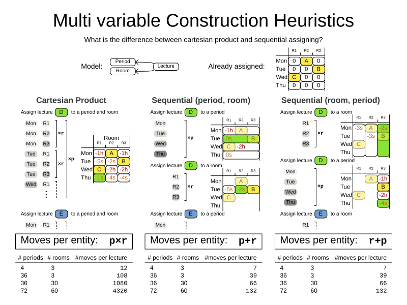
|
The order of the variables is important, especially in the sequential technique.
In the sequential example above, it’s better to select the Let the Benchmarker guide you. |
With three or more variables, it’s possible to combine the cartesian product and sequential techniques:
<constructionHeuristic>
<constructionHeuristicType>FIRST_FIT_DECREASING</constructionHeuristicType>
<cartesianProductMoveSelector>
<changeMoveSelector>
<valueSelector variableName="period"/>
</changeMoveSelector>
<changeMoveSelector>
<valueSelector variableName="room"/>
</changeMoveSelector>
</cartesianProductMoveSelector>
<changeMoveSelector>
<valueSelector variableName="teacher"/>
</changeMoveSelector>
</constructionHeuristic>12.13.3. Other scaling techniques in construction heuristics
Partitioned Search reduces the number of moves per step. On top of that, it runs the Construction Heuristic on the partitions in parallel. It is supported to only partition the Construction Heuristic phase.
Other Selector customizations can also reduce the number of moves generated by step:
13. Local search
13.1. Overview
Local Search starts from an initial solution and evolves that single solution into a mostly better and better solution. It uses a single search path of solutions, not a search tree. At each solution in this path it evaluates a number of moves on the solution and applies the most suitable move to take the step to the next solution. It does that for a high number of iterations until it’s terminated (usually because its time has run out).
Local Search acts a lot like a human planner: it uses a single search path and moves facts around to find a good feasible solution. Therefore it’s pretty natural to implement.
Local Search needs to start from an initialized solution, therefore it’s usually required to configure a Construction Heuristic phase before it.
13.2. Local search concepts
13.2.1. Step by step
A step is the winning Move.
Local Search tries a number of moves on the current solution and picks the best accepted move as the step:
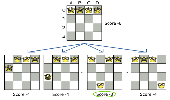
Because the move B0 to B3 has the highest score (-3), it is picked as the next step.
If multiple moves have the same highest score, one is picked randomly, in this case B0 to B3.
Note that C0 to C3 (not shown) could also have been picked because it also has the score -3.
The step is applied on the solution. From that new solution, Local Search tries every move again, to decide the next step after that. It continually does this in a loop, and we get something like this:
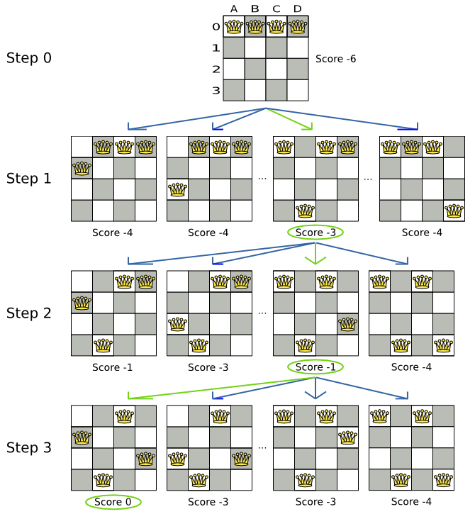
Notice that Local Search doesn’t use a search tree, but a search path. The search path is highlighted by the green arrows. At each step it tries all selected moves, but unless it’s the step, it doesn’t investigate that solution further. This is one of the reasons why Local Search is very scalable.
As shown above, Local Search solves the four queens problem by starting with the starting solution and make the following steps sequentially:
-
B0 to B3
-
D0 to D2
-
A0 to A1
Turn on debug logging for the category org.optaplanner to show those steps in the log:
INFO Solving started: time spent (0), best score (-6), environment mode (REPRODUCIBLE), random (JDK with seed 0).
DEBUG LS step (0), time spent (20), score (-3), new best score (-3), accepted/selected move count (12/12), picked move (Queen-1 {Row-0 -> Row-3}).
DEBUG LS step (1), time spent (31), score (-1), new best score (-1), accepted/selected move count (12/12), picked move (Queen-3 {Row-0 -> Row-2}).
DEBUG LS step (2), time spent (40), score (0), new best score (0), accepted/selected move count (12/12), picked move (Queen-0 {Row-0 -> Row-1}).
INFO Local Search phase (0) ended: time spent (41), best score (0), score calculation speed (5000/sec), step total (3).
INFO Solving ended: time spent (41), best score (0), score calculation speed (5000/sec), phase total (1), environment mode (REPRODUCIBLE).Notice that a log message includes the toString() method of the Move implementation which returns for example "Queen-1 {Row-0 → Row-3}".
A naive Local Search configuration solves the four queens problem in three steps, by evaluating only 37 possible solutions (three steps with 12 moves each + one starting solution), which is only a fraction of all 256 possible solutions. It solves 16 queens in 31 steps, by evaluating only 7441 out of 18446744073709551616 possible solutions. By using a Construction Heuristics phase first, it’s even a lot more efficient.
13.2.2. Decide the next step
Local Search decides the next step with the aid of three configurable components:
-
A
MoveSelectorwhich selects the possible moves of the current solution. See the chapter move and neighborhood selection. -
An
Acceptorwhich filters out unacceptable moves. -
A
Foragerwhich gathers accepted moves and picks the next step from them.
The solver phase configuration looks like this:
<localSearch>
<unionMoveSelector>
...
</unionMoveSelector>
<acceptor>
...
</acceptor>
<forager>
...
</forager>
</localSearch>In the example below, the MoveSelector generated the moves shown with the blue lines, the Acceptor accepted all of them and the Forager picked the move B0 to B3.
Turn on trace logging to show the decision making in the log:
INFO Solver started: time spent (0), score (-6), new best score (-6), random (JDK with seed 0).
TRACE Move index (0) not doable, ignoring move (Queen-0 {Row-0 -> Row-0}).
TRACE Move index (1), score (-4), accepted (true), move (Queen-0 {Row-0 -> Row-1}).
TRACE Move index (2), score (-4), accepted (true), move (Queen-0 {Row-0 -> Row-2}).
TRACE Move index (3), score (-4), accepted (true), move (Queen-0 {Row-0 -> Row-3}).
...
TRACE Move index (6), score (-3), accepted (true), move (Queen-1 {Row-0 -> Row-3}).
...
TRACE Move index (9), score (-3), accepted (true), move (Queen-2 {Row-0 -> Row-3}).
...
TRACE Move index (12), score (-4), accepted (true), move (Queen-3 {Row-0 -> Row-3}).
DEBUG LS step (0), time spent (6), score (-3), new best score (-3), accepted/selected move count (12/12), picked move (Queen-1 {Row-0 -> Row-3}).
...Because the last solution can degrade (for example in Tabu Search), the Solver remembers the best solution it has encountered through the entire search path.
Each time the current solution is better than the last best solution, the current solution is cloned and referenced as the new best solution.
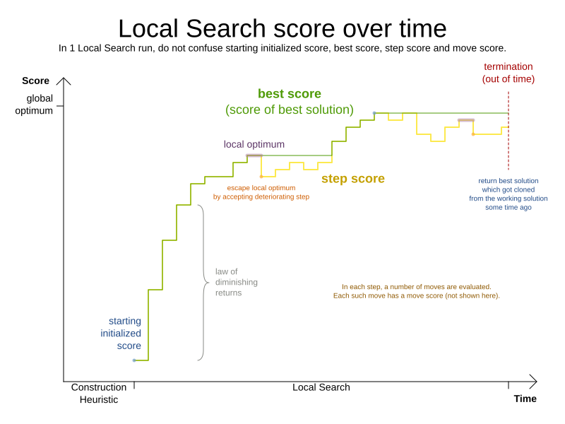
13.2.3. Acceptor
Use an Acceptor (together with a Forager) to activate Tabu Search, Simulated Annealing, Late Acceptance, … For each move it checks whether it is accepted or not.
By changing a few lines of configuration, you can easily switch from Tabu Search to Simulated Annealing or Late Acceptance and back.
You can implement your own Acceptor, but the built-in acceptors should suffice for most needs.
You can also combine multiple acceptors.
13.2.4. Forager
A Forager gathers all accepted moves and picks the move which is the next step.
Normally it picks the accepted move with the highest score.
If several accepted moves have the highest score, one is picked randomly to break the tie.
Breaking ties randomly leads to better results.
|
It is possible to disable breaking ties randomly by explicitly setting
|
13.2.4.1. Accepted count limit
When there are many possible moves, it becomes inefficient to evaluate all of them at every step. To evaluate only a random subset of all the moves, use:
-
An
acceptedCountLimitinteger, which specifies how many accepted moves should be evaluated during each step. By default, all accepted moves are evaluated at every step.<forager> <acceptedCountLimit>1000</acceptedCountLimit> </forager>
Unlike the n queens problem, real world problems require the use of acceptedCountLimit.
Start from an acceptedCountLimit that takes a step in less than two seconds. Turn on INFO logging to see the step times.
Use the Benchmarker to tweak the value.
|
With a low |
13.2.4.2. Pick early type
A forager can pick a move early during a step, ignoring subsequent selected moves. There are three pick early types for Local Search:
-
NEVER: A move is never picked early: all accepted moves are evaluated that the selection allows. This is the default.<forager> <pickEarlyType>NEVER</pickEarlyType> </forager> -
FIRST_BEST_SCORE_IMPROVING: Pick the first accepted move that improves the best score. If none improve the best score, it behaves exactly like the pickEarlyType NEVER.<forager> <pickEarlyType>FIRST_BEST_SCORE_IMPROVING</pickEarlyType> </forager> -
FIRST_LAST_STEP_SCORE_IMPROVING: Pick the first accepted move that improves the last step score. If none improve the last step score, it behaves exactly like the pickEarlyType NEVER.<forager> <pickEarlyType>FIRST_LAST_STEP_SCORE_IMPROVING</pickEarlyType> </forager>
13.3. Hill climbing (simple local search)
13.3.1. Algorithm description
Hill Climbing tries all selected moves and then takes the best move, which is the move which leads to the solution with the highest score. That best move is called the step move. From that new solution, it again tries all selected moves and takes the best move and continues like that iteratively. If multiple selected moves tie for the best move, one of them is randomly chosen as the best move.
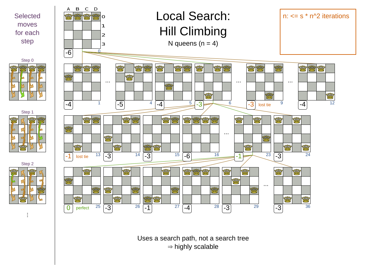
Notice that once a queen has moved, it can be moved again later. This is a good thing, because in an NP-complete problem it’s impossible to predict what will be the optimal final value for a planning variable.
13.3.2. Stuck in local optima
Hill climbing always takes improving moves. This may seem like a good thing, but it’s not: Hill Climbing can easily get stuck in a local optimum. This happens when it reaches a solution for which all the moves deteriorate the score. Even if it picks one of those moves, the next step might go back to the original solution and which case chasing its own tail:
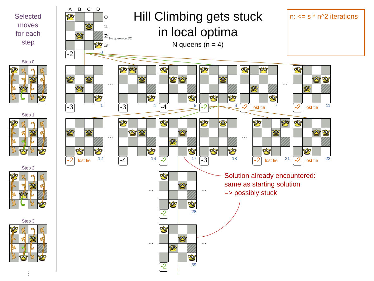
Improvements upon Hill Climbing (such as Tabu Search, Simulated Annealing and Late Acceptance) address the problem of being stuck in local optima. Therefore, it’s recommended to never use Hill Climbing, unless you’re absolutely sure there are no local optima in your planning problem.
13.3.3. Configuration
Simplest configuration:
<localSearch>
<localSearchType>HILL_CLIMBING</localSearchType>
</localSearch>Advanced configuration:
<localSearch>
...
<acceptor>
<acceptorType>HILL_CLIMBING</acceptorType>
</acceptor>
<forager>
<acceptedCountLimit>1</acceptedCountLimit>
</forager>
</localSearch>13.4. Tabu search
13.4.1. Algorithm description
Tabu Search is a Local Search that maintains a tabu list to avoid getting stuck in local optima. The tabu list holds recently used objects that are taboo to use for now. Moves that involve an object in the tabu list, are not accepted. The tabu list objects can be anything related to the move, such as the planning entity, planning value, move, solution, … Here’s an example with entity tabu for four queens, so the queens are put in the tabu list:
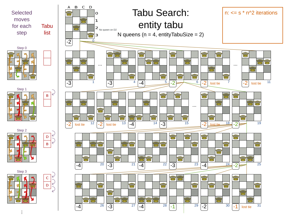
|
It’s called Tabu Search, not Taboo Search. There is no spelling error. |
Scientific paper: Tabu Search - Part 1 and Part 2 by Fred Glover (1989 - 1990)
13.4.2. Configuration
Simplest configuration:
<localSearch>
<localSearchType>TABU_SEARCH</localSearchType>
</localSearch>When Tabu Search takes steps it creates one or more tabus. For a number of steps, it does not accept a move if that move breaks tabu. That number of steps is the tabu size. Advanced configuration:
<localSearch>
...
<acceptor>
<entityTabuSize>7</entityTabuSize>
</acceptor>
<forager>
<acceptedCountLimit>1000</acceptedCountLimit>
</forager>
</localSearch>|
A Tabu Search acceptor should be combined with a high |
OptaPlanner implements several tabu types:
-
Planning entity tabu (recommended) makes the planning entities of recent steps tabu. For example, for N queens it makes the recently moved queens tabu. It’s recommended to start with this tabu type.
<acceptor> <entityTabuSize>7</entityTabuSize> </acceptor>To avoid hard coding the tabu size, configure a tabu ratio, relative to the number of entities, for example 2%:
<acceptor> <entityTabuRatio>0.02</entityTabuRatio> </acceptor> -
Planning value tabu makes the planning values of recent steps tabu. For example, for N queens it makes the recently moved to rows tabu.
<acceptor> <valueTabuSize>7</valueTabuSize> </acceptor>To avoid hard coding the tabu size, configure a tabu ratio, relative to the number of values, for example 2%:
<acceptor> <valueTabuRatio>0.02</valueTabuRatio> </acceptor> -
Move tabu makes recent steps tabu. It does not accept a move equal to one of those steps.
<acceptor> <moveTabuSize>7</moveTabuSize> </acceptor> -
Undo move tabu makes the undo move of recent steps tabu.
<acceptor> <undoMoveTabuSize>7</undoMoveTabuSize> </acceptor>
|
When using move tabu and undo move tabu with custom moves,
make sure that the planning entities do not include planning variables in their |
Sometimes it’s useful to combine tabu types:
<acceptor>
<entityTabuSize>7</entityTabuSize>
<valueTabuSize>3</valueTabuSize>
</acceptor>If the tabu size is too small, the solver can still get stuck in a local optimum. On the other hand, if the tabu size is too large, the solver can be inefficient by bouncing off the walls. Use the Benchmarker to fine tweak your configuration.
13.5. Simulated annealing
13.5.1. Algorithm description
Simulated Annealing evaluates only a few moves per step, so it steps quickly. In the classic implementation, the first accepted move is the winning step. A move is accepted if it doesn’t decrease the score or - in case it does decrease the score - it passes a random check. The chance that a decreasing move passes the random check decreases relative to the size of the score decrement and the time the phase has been running (which is represented as the temperature).
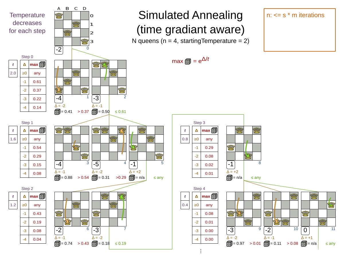
Simulated Annealing does not always pick the move with the highest score, neither does it evaluate many moves per step.
At least at first.
Instead, it gives non improving moves also a chance to be picked, depending on its score and the time gradient of the Termination.
In the end, it gradually turns into Hill Climbing, only accepting improving moves.
13.5.2. Configuration
Start with a simulatedAnnealingStartingTemperature set to the maximum score delta a single move can cause.
Use the Benchmarker to tweak the value.
Advanced configuration:
<localSearch>
...
<acceptor>
<simulatedAnnealingStartingTemperature>2hard/100soft</simulatedAnnealingStartingTemperature>
</acceptor>
<forager>
<acceptedCountLimit>1</acceptedCountLimit>
</forager>
</localSearch>Simulated Annealing should use a low acceptedCountLimit.
The classic algorithm uses an acceptedCountLimit of 1, but often 4 performs better.
Simulated Annealing can be combined with a tabu acceptor at the same time. That gives Simulated Annealing salted with a bit of Tabu. Use a lower tabu size than in a pure Tabu Search configuration.
<localSearch>
...
<acceptor>
<entityTabuSize>5</entityTabuSize>
<simulatedAnnealingStartingTemperature>2hard/100soft</simulatedAnnealingStartingTemperature>
</acceptor>
<forager>
<acceptedCountLimit>1</acceptedCountLimit>
</forager>
</localSearch>13.6. Late acceptance
13.6.1. Algorithm description
Late Acceptance (also known as Late Acceptance Hill Climbing) also evaluates only a few moves per step. A move is accepted if it does not decrease the score, or if it leads to a score that is at least the late score (which is the winning score of a fixed number of steps ago).
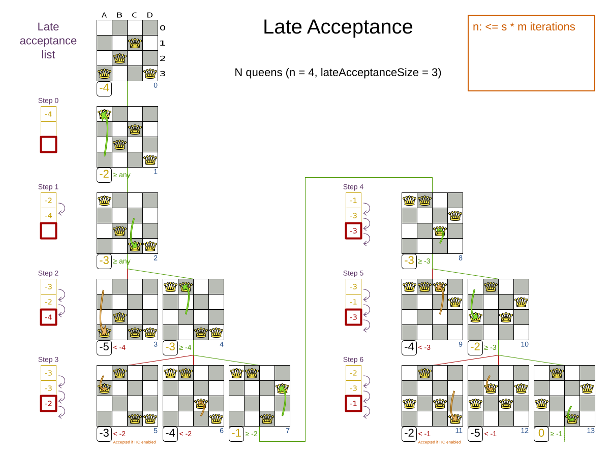
13.6.2. Configuration
Simplest configuration:
<localSearch>
<localSearchType>LATE_ACCEPTANCE</localSearchType>
</localSearch>Late Acceptance accepts any move that has a score which is higher than the best score of a number of steps ago.
That number of steps is the lateAcceptanceSize.
Advanced configuration:
<localSearch>
...
<acceptor>
<lateAcceptanceSize>400</lateAcceptanceSize>
</acceptor>
<forager>
<acceptedCountLimit>1</acceptedCountLimit>
</forager>
</localSearch>Late Acceptance should use a low acceptedCountLimit.
Late Acceptance can be combined with a tabu acceptor at the same time. That gives Late Acceptance salted with a bit of Tabu. Use a lower tabu size than in a pure Tabu Search configuration.
<localSearch>
...
<acceptor>
<entityTabuSize>5</entityTabuSize>
<lateAcceptanceSize>400</lateAcceptanceSize>
</acceptor>
<forager>
<acceptedCountLimit>1</acceptedCountLimit>
</forager>
</localSearch>13.7. Great Deluge
13.7.1. Algorithm description
Great Deluge algorithm is similar to the Simulated Annealing algorithm, it evaluates only a few moves per steps, so it steps quickly. The first accepted move is the winning step. A move is accepted only if it is not lower than the score value (water level) that we are working with. It means Great Deluge is deterministic and opposite of Simulated Annealing has no randomization in it. The water level is increased after every step either about the fixed value or by percentual value. A gradual increase in water level gives Great Deluge more time to escape from local maxima.
13.7.2. Configuration
Simplest configuration:
<localSearch>
<localSearchType>GREAT_DELUGE</localSearchType>
</localSearch>Great Deluge takes as starting water level best score from construction heuristic and uses default rain speed ratio. Advanced configuration:
<localSearch>
...
<acceptor>
<greatDelugeWaterLevelIncrementRatio>0.00000005</greatDelugeWaterLevelIncrementRatio>
</acceptor>
<forager>
<acceptedCountLimit>1</acceptedCountLimit>
</forager>
</localSearch>OptaPlanner implements two water level increment options:
If greatDelugeWaterLevelIncrementScore is set, the water level is increased by a constant value.
<acceptor>
<greatDelugeWaterLevelIncrementScore>10</greatDelugeWaterLevelIncrementScore>
</acceptor>To avoid hard coding the water level increment, configure a greatDelugeWaterLevelIncrementRatio (recommended) when the water level is increased by percentual value, so there is no need to know the size of the problem or value of a scoring function.
<acceptor>
<greatDelugeWaterLevelIncrementRatio>0.00000005</greatDelugeWaterLevelIncrementRatio>
</acceptor>The algorithm takes as starting value the best score from the construction heuristic. Use the Benchmarker to fine-tune tweak your configuration.
13.8. Step counting hill climbing
13.8.1. Algorithm description
Step Counting Hill Climbing also evaluates only a few moves per step. For a number of steps, it keeps the step score as a threshold. A move is accepted if it does not decrease the score, or if it leads to a score that is at least the threshold score.
13.8.2. Configuration
Step Counting Hill Climbing accepts any move that has a score which is higher than a threshold score.
Every number of steps (specified by stepCountingHillClimbingSize), the threshold score is set to the step score.
<localSearch>
...
<acceptor>
<stepCountingHillClimbingSize>400</stepCountingHillClimbingSize>
</acceptor>
<forager>
<acceptedCountLimit>1</acceptedCountLimit>
</forager>
</localSearch>Step Counting Hill Climbing should use a low acceptedCountLimit.
Step Counting Hill Climbing can be combined with a tabu acceptor at the same time, similar as shown in the Late Acceptance section.
13.9. Strategic oscillation
13.9.1. Algorithm description
Strategic Oscillation is an add-on, which works especially well with Tabu Search. Instead of picking the accepted move with the highest score, it employs a different mechanism: If there’s an improving move, it picks it. If there’s no improving move however, it prefers moves which improve a softer score level, over moves which break a harder score level less.
13.9.2. Configuration
Configure a finalistPodiumType, for example in a Tabu Search configuration:
<localSearch>
...
<acceptor>
<entityTabuSize>7</entityTabuSize>
</acceptor>
<forager>
<acceptedCountLimit>1000</acceptedCountLimit>
<finalistPodiumType>STRATEGIC_OSCILLATION</finalistPodiumType>
</forager>
</localSearch>The following finalistPodiumTypes are supported:
-
HIGHEST_SCORE(default): Pick the accepted move with the highest score. -
STRATEGIC_OSCILLATION: Alias for the default strategic oscillation variant. -
STRATEGIC_OSCILLATION_BY_LEVEL: If there is an accepted improving move, pick it. If no such move exists, prefer an accepted move which improves a softer score level over one that doesn’t (even if it has a better harder score level). A move is improving if it’s better than the last completed step score. -
STRATEGIC_OSCILLATION_BY_LEVEL_ON_BEST_SCORE: LikeSTRATEGIC_OSCILLATION_BY_LEVEL, but define improving as better than the best score (instead of the last completed step score).
13.10. Variable neighborhood descent
13.10.1. Algorithm description
Variable Neighborhood Descent iteratively tries multiple move selectors in original order (depleting each selector entirely before trying the next one), picking the first improving move (which also resets the iterator back to the first move selector).
|
Despite that VND has a name that ends with descent (from the research papers), the implementation will ascend to a higher score (which is a better score). |
13.10.2. Configuration
Simplest configuration:
<localSearch>
<localSearchType>VARIABLE_NEIGHBORHOOD_DESCENT</localSearchType>
</localSearch>Advanced configuration:
<localSearch>
<unionMoveSelector>
<selectionOrder>ORIGINAL</selectionOrder>
<changeMoveSelector/>
<swapMoveSelector/>
...
</unionMoveSelector>
<acceptor>
<acceptorType>HILL_CLIMBING</acceptorType>
</acceptor>
<forager>
<pickEarlyType>FIRST_LAST_STEP_SCORE_IMPROVING</pickEarlyType>
</forager>
</localSearch>Variable Neighborhood Descent doesn’t scale well, but it is useful in some use cases with a very erratic score landscape.
14. Evolutionary algorithms
14.1. Overview
Evolutionary Algorithms work on a population of solutions and evolve that population.
14.2. Evolutionary strategies
This algorithm has not been implemented yet.
14.3. Genetic algorithms
This algorithm has not been implemented yet.
|
A good Genetic Algorithms prototype in OptaPlanner was written some time ago, but it wasn’t practical to merge and support it at the time. The results of Genetic Algorithms were consistently and seriously inferior to all the Local Search variants (except Hill Climbing) on all use cases tried. Nevertheless, a future version of OptaPlanner will add support for Genetic Algorithms, so you can easily benchmark Genetic Algorithms on your use case too. |
15. Hyperheuristics
15.1. Overview
A hyperheuristic automates the decision which heuristic(s) to use on a specific data set.
A future version of OptaPlanner will have native support for hyperheuristics.
Meanwhile, it’s possible to implement it yourself: Based on the size or difficulty of a data set (which is a criterion), use a different Solver configuration (or adjust the default configuration using the Solver configuration API). The Benchmarker can help to identify such criteria.
16. Partitioned search
16.1. Algorithm description
It is often more efficient to partition large data sets (usually above 5000 planning entities) into smaller pieces and solve them separately. Partition Search is multithreaded, so it provides a performance boost on multi-core machines due to higher CPU utilization. Additionally, even when only using one CPU, it finds an initial solution faster, because the search space sum of a partitioned Construction Heuristic is far less than its non-partitioned variant.
However, partitioning does lead to suboptimal results, even if the pieces are solved optimally, as shown below:
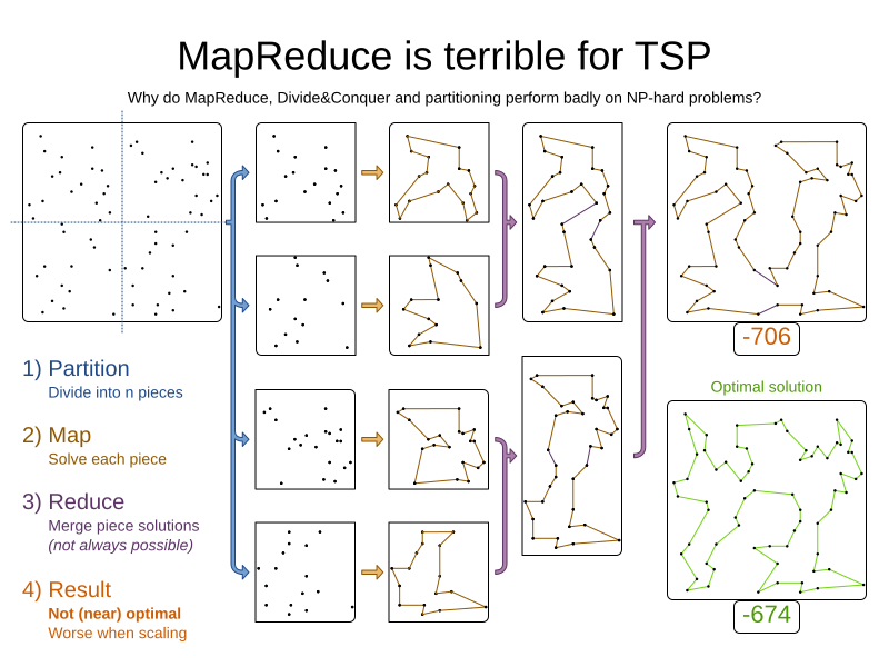
It effectively trades a short term gain in solution quality for long term loss. One way to compensate for this loss, is to run a non-partitioned Local Search after the Partitioned Search phase.
|
Not all use cases can be partitioned. Partitioning only works for use cases where the planning entities and value ranges can be split into n partitions, without any of the constraints crossing boundaries between partitions. |
16.2. Configuration
Simplest configuration:
<partitionedSearch>
<solutionPartitionerClass>org.optaplanner.examples.cloudbalancing.optional.partitioner.CloudBalancePartitioner</solutionPartitionerClass>
</partitionedSearch>Also add a @PlanningId annotations on every planning entity class and planning value class. There are several ways to partition a solution.
Advanced configuration:
<partitionedSearch>
...
<solutionPartitionerClass>org.optaplanner.examples.cloudbalancing.optional.partitioner.CloudBalancePartitioner</solutionPartitionerClass>
<runnablePartThreadLimit>4</runnablePartThreadLimit>
<constructionHeuristic>...</constructionHeuristic>
<localSearch>...</localSearch>
</partitionedSearch>The runnablePartThreadLimit allows limiting CPU usage to avoid hanging your machine, see below.
To run in an environment that doesn’t like arbitrary thread creation, plug in a custom thread factory.
|
A logging level of |
Just like a <solver> element, the <partitionedSearch> element can contain one or more phases.
Each of those phases will be run on each partition.
A common configuration is to first run a Partitioned Search phase (which includes a Construction Heuristic and a Local Search) followed by a non-partitioned Local Search phase:
<partitionedSearch>
<solutionPartitionerClass>...CloudBalancePartitioner</solutionPartitionerClass>
<constructionHeuristic/>
<localSearch>
<termination>
<secondsSpentLimit>60</secondsSpentLimit>
</termination>
</localSearch>
</partitionedSearch>
<localSearch/>16.3. Partitioning a solution
16.3.1. Custom SolutionPartitioner
To use a custom SolutionPartitioner, configure one on the Partitioned Search phase:
<partitionedSearch>
<solutionPartitionerClass>org.optaplanner.examples.cloudbalancing.optional.partitioner.CloudBalancePartitioner</solutionPartitionerClass>
</partitionedSearch>Implement the SolutionPartitioner interface:
public interface SolutionPartitioner<Solution_> {
List<Solution_> splitWorkingSolution(ScoreDirector<Solution_> scoreDirector, Integer runnablePartThreadLimit);
}The size() of the returned List is the partCount (the number of partitions).
This can be decided dynamically, for example, based on the size of the non-partitioned solution.
The partCount is unrelated to the runnablePartThreadLimit.
For example:
public class CloudBalancePartitioner implements SolutionPartitioner<CloudBalance> {
private int partCount = 4;
private int minimumProcessListSize = 75;
@Override
public List<CloudBalance> splitWorkingSolution(ScoreDirector<CloudBalance> scoreDirector, Integer runnablePartThreadLimit) {
CloudBalance originalSolution = scoreDirector.getWorkingSolution();
List<CloudComputer> originalComputerList = originalSolution.getComputerList();
List<CloudProcess> originalProcessList = originalSolution.getProcessList();
int partCount = this.partCount;
if (originalProcessList.size() / partCount < minimumProcessListSize) {
partCount = originalProcessList.size() / minimumProcessListSize;
}
List<CloudBalance> partList = new ArrayList<>(partCount);
for (int i = 0; i < partCount; i++) {
CloudBalance partSolution = new CloudBalance(originalSolution.getId(),
new ArrayList<>(originalComputerList.size() / partCount + 1),
new ArrayList<>(originalProcessList.size() / partCount + 1));
partList.add(partSolution);
}
int partIndex = 0;
Map<Long, Pair<Integer, CloudComputer>> idToPartIndexAndComputerMap = new HashMap<>(originalComputerList.size());
for (CloudComputer originalComputer : originalComputerList) {
CloudBalance part = partList.get(partIndex);
CloudComputer computer = new CloudComputer(
originalComputer.getId(),
originalComputer.getCpuPower(), originalComputer.getMemory(),
originalComputer.getNetworkBandwidth(), originalComputer.getCost());
part.getComputerList().add(computer);
idToPartIndexAndComputerMap.put(computer.getId(), Pair.of(partIndex, computer));
partIndex = (partIndex + 1) % partList.size();
}
partIndex = 0;
for (CloudProcess originalProcess : originalProcessList) {
CloudBalance part = partList.get(partIndex);
CloudProcess process = new CloudProcess(
originalProcess.getId(),
originalProcess.getRequiredCpuPower(), originalProcess.getRequiredMemory(),
originalProcess.getRequiredNetworkBandwidth());
part.getProcessList().add(process);
if (originalProcess.getComputer() != null) {
Pair<Integer, CloudComputer> partIndexAndComputer = idToPartIndexAndComputerMap.get(
originalProcess.getComputer().getId());
if (partIndexAndComputer == null) {
throw new IllegalStateException("The initialized process (" + originalProcess
+ ") has a computer (" + originalProcess.getComputer()
+ ") which doesn't exist in the originalSolution (" + originalSolution + ").");
}
if (partIndex != partIndexAndComputer.getLeft().intValue()) {
throw new IllegalStateException("The initialized process (" + originalProcess
+ ") with partIndex (" + partIndex
+ ") has a computer (" + originalProcess.getComputer()
+ ") which belongs to another partIndex (" + partIndexAndComputer.getLeft() + ").");
}
process.setComputer(partIndexAndComputer.getRight());
}
partIndex = (partIndex + 1) % partList.size();
}
return partList;
}
}To configure values of a SolutionPartitioner dynamically in the solver configuration
(so the Benchmarker can tweak those parameters),
add the solutionPartitionerCustomProperties element and use custom properties:
<partitionedSearch>
<solutionPartitionerClass>...CloudBalancePartitioner</solutionPartitionerClass>
<solutionPartitionerCustomProperties>
<property name="myPartCount" value="8"/>
<property name="myMinimumProcessListSize" value="100"/>
</solutionPartitionerCustomProperties>
</partitionedSearch>16.4. Runnable part thread limit
When running a multithreaded solver, such as Partitioned Search, CPU power can quickly become a scarce resource, which can cause other processes or threads to hang or freeze. However, OptaPlanner has a system to prevent CPU starving of other processes (such as an SSH connection in production or your IDE in development) or other threads (such as the servlet threads that handle REST requests).
As explained in sizing hardware and software,
each solver (including each child solver) does no IO during solve() and therefore saturates one CPU core completely.
In Partitioned Search, every partition always has its own thread, called a part thread.
It is impossible for two partitions to share a thread,
because of asynchronous termination: the second thread would never run.
Every part thread will try to consume one CPU core entirely, so if there are more partitions than CPU cores,
this will probably hang the system.
Thread.setPriority() is often too weak to solve this hogging problem, so another approach is used.
The runnablePartThreadLimit parameter specifies how many part threads are runnable at the same time.
The other part threads will temporarily block and therefore will not consume any CPU power.
This parameter basically specifies how many CPU cores are donated to OptaPlanner.
All part threads share the CPU cores in a round-robin manner
to consume (more or less) the same number of CPU cycles:
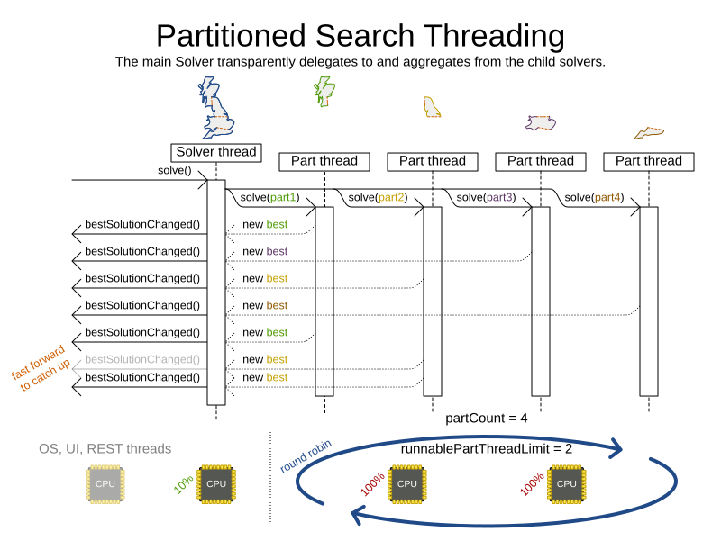
The following runnablePartThreadLimit options are supported:
-
UNLIMITED: Allow OptaPlanner to occupy all CPU cores, do not avoid hogging. Useful if a no hogging CPU policy is configured on the OS level. -
AUTO(default): Let OptaPlanner decide how many CPU cores to occupy. This formula is based on experience. It does not hog all CPU cores on a multi-core machine. -
Static number: The number of CPU cores to consume. For example:
<runnablePartThreadLimit>2</runnablePartThreadLimit>
|
If the |
17. Benchmarking and tweaking
17.1. Find the best solver configuration
OptaPlanner supports several optimization algorithms, so you’re probably wondering which is the best one? Although some optimization algorithms generally perform better than others, it really depends on your problem domain. Most solver phases have parameters which can be tweaked. Those parameters can influence the results a lot, even though most solver phases work pretty well out-of-the-box.
Luckily, OptaPlanner includes a benchmarker, which allows you to play out different solver phases with different settings against each other in development, so you can use the best configuration for your planning problem in production.
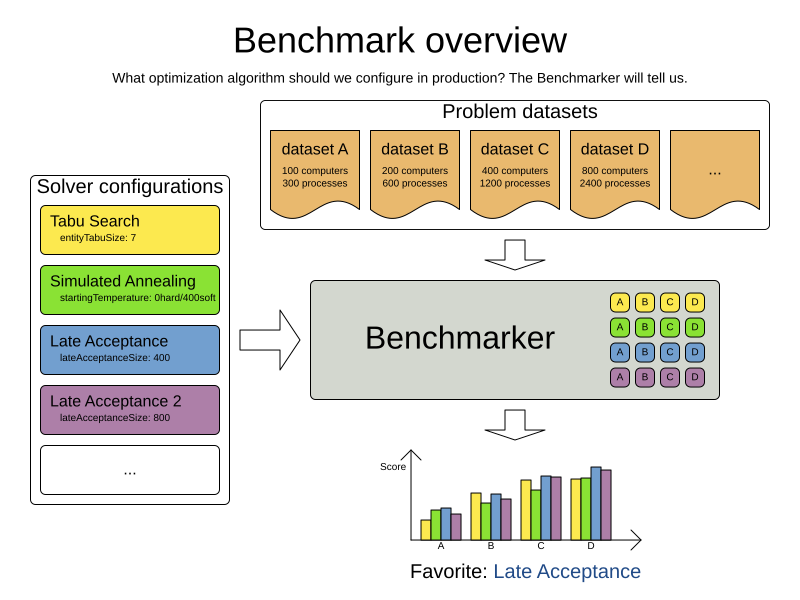
17.2. Benchmark configuration
17.2.1. Add a dependency on optaplanner-benchmark
The benchmarker is in a separate artifact called optaplanner-benchmark.
If you use Maven, add a dependency in your pom.xml file:
<dependency>
<groupId>org.optaplanner</groupId>
<artifactId>optaplanner-benchmark</artifactId>
</dependency>This is similar for Gradle, Ivy and Buildr.
The version must be exactly the same as the optaplanner-core version used (which is automatically the case if you import optaplanner-bom).
If you use ANT, you’ve probably already copied the required jars from the download zip’s binaries directory.
17.2.2. Run a simple benchmark
To quickly setup a benchmark, create a PlannerBenchmarkFactory from your solver configuration XML,
load a few datasets and benchmark them. For example, with 3 datasets:
PlannerBenchmarkFactory benchmarkFactory = PlannerBenchmarkFactory.createFromSolverConfigXmlResource(
"org/optaplanner/examples/cloudbalancing/solver/cloudBalancingSolverConfig.xml");
CloudBalance dataset1 = ...;
CloudBalance dataset2 = ...;
CloudBalance dataset3 = ...;
PlannerBenchmark benchmark = benchmarkFactory.buildPlannerBenchmark(
dataset1, dataset2, dataset3);
benchmark.benchmarkAndShowReportInBrowser();This generates a benchmark report in local/benchmarkReport and shows it in your browser when it’s finished.
The SolverFactory's solver configuration needs a termination to limit how long each dataset runs.
To configure a different benchmark directory, pass a File parameter to createFromSolverConfigXmlResource().
The generated benchmark report already contains interesting information, but it doesn’t compare solver configurations to find the best algorithm. To do that, set up an explicit benchmark configuration:
17.2.3. Configure and run an advanced benchmark
Build a PlannerBenchmark instance with a PlannerBenchmarkFactory.
Configure it with a benchmark configuration XML file, provided as a classpath resource:
PlannerBenchmarkFactory benchmarkFactory = PlannerBenchmarkFactory.createFromXmlResource(
"org/optaplanner/examples/cloudbalancing/benchmark/cloudBalancingBenchmarkConfig.xml");
PlannerBenchmark benchmark = benchmarkFactory.buildPlannerBenchmark();
benchmark.benchmarkAndShowReportInBrowser();Alternatively, create a PlannerBenchmarkFactory programmatically from a PlannerBenchmarkConfig.
A benchmark configuration XML file looks like this:
<?xml version="1.0" encoding="UTF-8"?>
<plannerBenchmark xmlns="https://www.optaplanner.org/xsd/benchmark" xmlns:xsi="http://www.w3.org/2001/XMLSchema-instance"
xsi:schemaLocation="https://www.optaplanner.org/xsd/benchmark https://www.optaplanner.org/xsd/benchmark/benchmark.xsd">
<benchmarkDirectory>local/data/nqueens</benchmarkDirectory>
<inheritedSolverBenchmark>
<solver>
...<!-- Common solver configuration -->
</solver>
<problemBenchmarks>
...
<inputSolutionFile>data/cloudbalancing/unsolved/100computers-300processes.json</inputSolutionFile>
<inputSolutionFile>data/cloudbalancing/unsolved/200computers-600processes.json</inputSolutionFile>
</problemBenchmarks>
</inheritedSolverBenchmark>
<solverBenchmark>
<name>Tabu Search</name>
<solver>
...<!-- Tabu Search specific solver configuration -->
</solver>
</solverBenchmark>
<solverBenchmark>
<name>Simulated Annealing</name>
<solver>
...<!-- Simulated Annealing specific solver configuration -->
</solver>
</solverBenchmark>
<solverBenchmark>
<name>Late Acceptance</name>
<solver>
...<!-- Late Acceptance specific solver configuration -->
</solver>
</solverBenchmark>
</plannerBenchmark>This PlannerBenchmark tries three configurations (Tabu Search, Simulated Annealing and Late Acceptance)
on two data sets (100computers-300processes and 200computers-600processes), so it runs six solvers.
Every <solverBenchmark> element contains a solver configuration and one or more <inputSolutionFile> elements.
It runs the solver configuration on each of those unsolved solution files.
The element name is optional, because it is generated if absent.
The inputSolutionFile is read by a SolutionFileIO, relative to the working directory.
|
Use a forward slash ( Do not use backslash ( |
The benchmark report is written in the directory specified by the <benchmarkDirectory> element (relative to the working directory).
|
It’s recommended that the |
If an Exception or Error occurs in a single benchmark, the entire Benchmarker does not fail-fast (unlike everything else in OptaPlanner).
Instead, the Benchmarker continues to run all other benchmarks, write the benchmark report and then fail (if there is at least one failing single benchmark).
The failing benchmarks are clearly marked as such in the benchmark report.
17.2.3.1. Inherited solver benchmark
To lower verbosity, the common parts of multiple <solverBenchmark> elements are extracted to the <inheritedSolverBenchmark> element.
Every property can still be overwritten per <solverBenchmark> element.
Note that inherited solver phases such as <constructionHeuristic> or <localSearch> are not overwritten
but instead are added to the tail of the solver phases list.
17.2.4. SolutionFileIO: input and output of solution files
17.2.4.1. SolutionFileIO interface
The benchmarker needs to be able to read the input files to load a problem.
Also, it optionally writes the best solution of each benchmark to an output file.
It does that through the SolutionFileIO interface which has a read and write method:
public interface SolutionFileIO<Solution_> {
...
Solution_ read(File inputSolutionFile);
void write(Solution_ solution, File outputSolutionFile);
}The SolutionFileIO interface is in the optaplanner-persistence-common jar (which is a dependency of the optaplanner-benchmark jar).
There are several ways to serialize a solution.
17.2.4.2. JacksonSolutionFileIO: serialize to and from an JSON format
To read and write solutions in JSON format via Jackson, extend the JacksonSolutionFileIO:
public class NQueensJsonSolutionFileIO extends JacksonSolutionFileIO<NQueens> {
public NQueensJsonSolutionFileIO() {
// NQueens is the @PlanningSolution class.
super(NQueens.class);
}
}If the JSON file requires specific Jackson modules and features to be enabled/disabled. You could create your desired object mapper as a dependency to the JacksonSolutionFileIO as follows:
public class NQueensJsonSolutionFileIO extends JacksonSolutionFileIO<NQueens> {
public NQueensJsonSolutionFileIO() {
// NQueens is the @PlanningSolution class.
super(NQueens.class,
new ObjectMapper()
.registerModule(new JavaTimeModule())
.disable(SerializationFeature.WRITE_DATES_AS_TIMESTAMPS)
);
}
}Then use it in the benchmark configuration like so:
<problemBenchmarks>
<solutionFileIOClass>org.optaplanner.examples.nqueens.persistence.NQueensJsonSolutionFileIO</solutionFileIOClass>
<inputSolutionFile>data/nqueens/unsolved/32queens.json</inputSolutionFile>
...
</problemBenchmarks>17.2.4.3. JaxbSolutionFileIO: serialize to and from an XML format
To read and write solutions in the XML format via Java Architecture for XML Binding (JAXB), extend the JaxbSolutionFileIO:
public class NQueensXmlSolutionFileIO extends JaxbSolutionFileIO<NQueens> {
public NQueensXmlSolutionFileIO() {
// NQueens is the @PlanningSolution class.
super(NQueens.class);
}
}and use it in the benchmark configuration:
<problemBenchmarks>
<solutionFileIOClass>org.optaplanner.examples.nqueens.persistence.NQueensSolutionFileIO</solutionFileIOClass>
<inputSolutionFile>data/nqueens/unsolved/32queens.xml</inputSolutionFile>
...
</problemBenchmarks>Add JAXB annotations (such as @XmlElement) on your domain classes to use a less verbose XML format.
Regardless, XML is still a very verbose format.
Reading or writing large datasets in this format can cause an OutOfMemoryError, StackOverflowError
or large performance degradation.
17.2.4.4. Custom SolutionFileIO: serialize to and from a custom format
Implement your own SolutionFileIO implementation and configure it with the solutionFileIOClass element to write to a custom format (such as a txt or a binary format):
<problemBenchmarks>
<solutionFileIOClass>org.optaplanner.examples.machinereassignment.persistence.MachineReassignmentFileIO</solutionFileIOClass>
<inputSolutionFile>data/machinereassignment/import/model_a1_1.txt</inputSolutionFile>
...
</problemBenchmarks>It’s recommended that output files can be read as input files,
which implies that getInputFileExtension() and getOutputFileExtension() return the same value.
|
A |
17.2.4.5. Reading an input solution from a database or other storage
There are two options if your dataset is in a relational database or another type of repository:
-
Extract the datasets from the database and serialize them to a local file, for example as JSON with
JacksonSolutionFileIO. Then use those files in<inputSolutionFile>elements.-
The benchmarks are now more reliable because they run offline.
-
Each dataset is only loaded just in time.
-
-
Load all the datasets in advance and pass them to the
buildPlannerBenchmark()method:PlannerBenchmark plannerBenchmark = benchmarkFactory.buildPlannerBenchmark(dataset1, dataset2, dataset3);
17.2.5. Warming up the HotSpot compiler
Without a warm up, the results of the first (or first few) benchmarks are not reliable because they lose CPU time on HotSpot JIT compilation.
To avoid that distortion, the benchmarker runs some of the benchmarks for 30 seconds, before running the real benchmarks. That default warm up of 30 seconds usually suffices. Change it, for example to give it 60 seconds:
<plannerBenchmark xmlns="https://www.optaplanner.org/xsd/benchmark" xmlns:xsi="http://www.w3.org/2001/XMLSchema-instance"
xsi:schemaLocation="https://www.optaplanner.org/xsd/benchmark https://www.optaplanner.org/xsd/benchmark/benchmark.xsd">
...
<warmUpSecondsSpentLimit>60</warmUpSecondsSpentLimit>
...
</plannerBenchmark>Turn off the warm up phase altogether by setting it to zero:
<plannerBenchmark xmlns="https://www.optaplanner.org/xsd/benchmark" xmlns:xsi="http://www.w3.org/2001/XMLSchema-instance"
xsi:schemaLocation="https://www.optaplanner.org/xsd/benchmark https://www.optaplanner.org/xsd/benchmark/benchmark.xsd">
...
<warmUpSecondsSpentLimit>0</warmUpSecondsSpentLimit>
...
</plannerBenchmark>|
The warm up time budget does not include the time it takes to load the datasets. With large datasets, this can cause the warm up to run considerably longer than specified in the configuration. |
17.2.6. Benchmark blueprint: a predefined configuration
To quickly configure and run a benchmark for typical solver configs, use a solverBenchmarkBluePrint instead of solverBenchmarks:
<?xml version="1.0" encoding="UTF-8"?>
<plannerBenchmark xmlns="https://www.optaplanner.org/xsd/benchmark" xmlns:xsi="http://www.w3.org/2001/XMLSchema-instance"
xsi:schemaLocation="https://www.optaplanner.org/xsd/benchmark https://www.optaplanner.org/xsd/benchmark/benchmark.xsd">
<benchmarkDirectory>local/data/nqueens</benchmarkDirectory>
<inheritedSolverBenchmark>
<solver>
<solutionClass>org.optaplanner.examples.nqueens.domain.NQueens</solutionClass>
<entityClass>org.optaplanner.examples.nqueens.domain.Queen</entityClass>
<scoreDirectorFactory>
<constraintProviderClass>org.optaplanner.examples.nqueens.score.NQueensConstraintProvider</constraintProviderClass>
<initializingScoreTrend>ONLY_DOWN</initializingScoreTrend>
</scoreDirectorFactory>
<termination>
<minutesSpentLimit>1</minutesSpentLimit>
</termination>
</solver>
<problemBenchmarks>
<solutionFileIOClass>org.optaplanner.examples.nqueens.persistence.NQueensSolutionFileIO</solutionFileIOClass>
<inputSolutionFile>data/nqueens/unsolved/32queens.json</inputSolutionFile>
<inputSolutionFile>data/nqueens/unsolved/64queens.json</inputSolutionFile>
</problemBenchmarks>
</inheritedSolverBenchmark>
<solverBenchmarkBluePrint>
<solverBenchmarkBluePrintType>EVERY_CONSTRUCTION_HEURISTIC_TYPE_WITH_EVERY_LOCAL_SEARCH_TYPE</solverBenchmarkBluePrintType>
</solverBenchmarkBluePrint>
</plannerBenchmark>The following SolverBenchmarkBluePrintTypes are supported:
-
CONSTRUCTION_HEURISTIC_WITH_AND_WITHOUT_LOCAL_SEARCH: Run the default Construction Heuristic type with and without the default Local Search type. -
EVERY_CONSTRUCTION_HEURISTIC_TYPE: Run every Construction Heuristic type (First Fit, First Fit Decreasing, Cheapest Insertion, …). -
EVERY_LOCAL_SEARCH_TYPE: Run every Local Search type (Tabu Search, Late Acceptance, …) with the default Construction Heuristic. -
EVERY_CONSTRUCTION_HEURISTIC_TYPE_WITH_EVERY_LOCAL_SEARCH_TYPE: Run every Construction Heuristic type with every Local Search type.
17.2.7. Write the output solution of benchmark runs
The best solution of each benchmark run can be written in the benchmarkDirectory.
By default, this is disabled, because the files are rarely used and considered bloat.
Also, on large datasets, writing the best solution of each single benchmark can take quite some time and memory (causing an OutOfMemoryError), especially in a verbose format like XML.
To write those solutions in the benchmarkDirectory, enable writeOutputSolutionEnabled:
<problemBenchmarks>
...
<writeOutputSolutionEnabled>true</writeOutputSolutionEnabled>
...
</problemBenchmarks>17.2.8. Benchmark logging
Benchmark logging is configured like solver logging.
To separate the log messages of each single benchmark run into a separate file, use the MDC with key subSingleBenchmark.name in a sifting appender.
For example with Logback in logback.xml:
<appender name="fileAppender" class="ch.qos.logback.classic.sift.SiftingAppender">
<discriminator>
<key>subSingleBenchmark.name</key>
<defaultValue>app</defaultValue>
</discriminator>
<sift>
<appender name="fileAppender.${subSingleBenchmark.name}" class="...FileAppender">
<file>local/log/optaplannerBenchmark-${subSingleBenchmark.name}.log</file>
...
</appender>
</sift>
</appender>17.3. Benchmark report
17.3.1. HTML report
After running a benchmark, an HTML report will be written in the benchmarkDirectory with the index.html filename.
Open it in your browser.
It has a nice overview of your benchmark including:
-
Summary statistics: graphs and tables
-
Problem statistics per
inputSolutionFile: graphs and CSV -
Each solver configuration (ranked): Handy to copy and paste
-
Benchmark information: settings, hardware, …
|
Graphs are generated by the excellent JFreeChart library. |
The HTML report will use your default locale to format numbers.
If you share the benchmark report with people from another country, consider overwriting the locale accordingly:
<plannerBenchmark xmlns="https://www.optaplanner.org/xsd/benchmark" xmlns:xsi="http://www.w3.org/2001/XMLSchema-instance"
xsi:schemaLocation="https://www.optaplanner.org/xsd/benchmark https://www.optaplanner.org/xsd/benchmark/benchmark.xsd">
...
<benchmarkReport>
<locale>en_US</locale>
</benchmarkReport>
...
</plannerBenchmark>17.3.2. Ranking the solvers
The benchmark report automatically ranks the solvers.
The Solver with rank 0 is called the favorite Solver: it performs best overall, but it might not be the best on every problem.
It’s recommended to use that favorite Solver in production.
However, there are different ways of ranking the solvers. Configure it like this:
<plannerBenchmark xmlns="https://www.optaplanner.org/xsd/benchmark" xmlns:xsi="http://www.w3.org/2001/XMLSchema-instance"
xsi:schemaLocation="https://www.optaplanner.org/xsd/benchmark https://www.optaplanner.org/xsd/benchmark/benchmark.xsd">
...
<benchmarkReport>
<solverRankingType>TOTAL_SCORE</solverRankingType>
</benchmarkReport>
...
</plannerBenchmark>The following solverRankingTypes are supported:
-
TOTAL_SCORE(default): Maximize the overall score, so minimize the overall cost if all solutions would be executed. -
WORST_SCORE: Minimize the worst case scenario. -
TOTAL_RANKING: Maximize the overall ranking. Use this if your datasets differ greatly in size or difficulty, producing a difference inScoremagnitude.
Solvers with at least one failed single benchmark do not get a ranking.
Solvers with not fully initialized solutions are ranked worse.
To use a custom ranking, implement a Comparator:
<benchmarkReport>
<solverRankingComparatorClass>...TotalScoreSolverRankingComparator</solverRankingComparatorClass>
</benchmarkReport>Or by implementing a weight factory:
<benchmarkReport>
<solverRankingWeightFactoryClass>...TotalRankSolverRankingWeightFactory</solverRankingWeightFactoryClass>
</benchmarkReport>17.4. Summary statistics
17.4.1. Best score summary (graph and table)
Shows the best score per inputSolutionFile for each solver configuration.
Useful for visualizing the best solver configuration.
17.4.2. Best score scalability summary (graph)
Shows the best score per problem scale for each solver configuration.
Useful for visualizing the scalability of each solver configuration.
|
The problem scale will report |
17.4.3. Best score distribution summary (graph)
Shows the best score distribution per inputSolutionFile for each solver configuration.
Useful for visualizing the reliability of each solver configuration.
Enable statistical benchmarking to use this summary.
17.4.4. Winning score difference summary (graph And table)
Shows the winning score difference per inputSolutionFile for each solver configuration.
The winning score difference is the score difference with the score of the winning solver configuration for that particular inputSolutionFile.
Useful for zooming in on the results of the best score summary.
17.4.5. Worst score difference percentage (ROI) summary (graph And table)
Shows the return on investment (ROI) per inputSolutionFile for each solver configuration if you’d upgrade from the worst solver configuration for that particular inputSolutionFile.
Useful for visualizing the return on investment (ROI) to decision makers.
17.4.6. Score calculation speed summary (graph And table)
Shows the score calculation speed: a count per second per problem scale for each solver configuration.
Useful for comparing different score calculators and/or constraint implementations (presuming that the solver configurations do not differ otherwise). Also useful to measure the scalability cost of an extra constraint.
17.4.7. Time spent summary (graph And table)
Shows the time spent per inputSolutionFile for each solver configuration.
This is pointless if it’s benchmarking against a fixed time limit.
Useful for visualizing the performance of construction heuristics (presuming that no other solver phases are configured).
17.4.8. Time spent scalability summary (graph)
Shows the time spent per problem scale for each solver configuration. This is pointless if it’s benchmarking against a fixed time limit.
Useful for extrapolating the scalability of construction heuristics (presuming that no other solver phases are configured).
17.4.9. Best score per time spent summary (graph)
Shows the best score per time spent for each solver configuration. This is pointless if it’s benchmarking against a fixed time limit.
Useful for visualizing trade-off between the best score versus the time spent for construction heuristics (presuming that no other solver phases are configured).
17.5. Statistic per dataset (graph and CSV)
17.5.1. Enable a problem statistic
The benchmarker supports outputting problem statistics as graphs and CSV (comma separated values) files to the benchmarkDirectory.
To configure one or more, add a problemStatisticType line for each one:
<plannerBenchmark xmlns="https://www.optaplanner.org/xsd/benchmark" xmlns:xsi="http://www.w3.org/2001/XMLSchema-instance"
xsi:schemaLocation="https://www.optaplanner.org/xsd/benchmark https://www.optaplanner.org/xsd/benchmark/benchmark.xsd">
<benchmarkDirectory>local/data/nqueens/solved</benchmarkDirectory>
<inheritedSolverBenchmark>
<problemBenchmarks>
...
<problemStatisticType>BEST_SCORE</problemStatisticType>
<problemStatisticType>SCORE_CALCULATION_SPEED</problemStatisticType>
</problemBenchmarks>
...
</inheritedSolverBenchmark>
...
</plannerBenchmark>|
These problem statistics can slow down the solvers noticeably, which affects the benchmark results.
That’s why they are optional and only The summary statistics do not slow down the solver and are always generated. |
The following types are supported:
17.5.2. Best score over time statistic (graph and CSV)
Shows how the best score evolves over time. It is run by default. To run it when other statistics are configured, also add:
<problemBenchmarks>
...
<problemStatisticType>BEST_SCORE</problemStatisticType>
</problemBenchmarks>
|
A time gradient based algorithm (such as Simulated Annealing) will have a different statistic if it’s run with a different time limit configuration. That’s because this Simulated Annealing implementation automatically determines its velocity based on the amount of time that can be spent. On the other hand, for the Tabu Search and Late Acceptance, what you see is what you’d get. |
The best score over time statistic is very useful to detect abnormalities, such as a potential score trap which gets the solver temporarily stuck in a local optima.
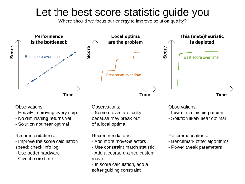
17.5.3. Step score over time statistic (graph and CSV)
To see how the step score evolves over time, add:
<problemBenchmarks>
...
<problemStatisticType>STEP_SCORE</problemStatisticType>
</problemBenchmarks>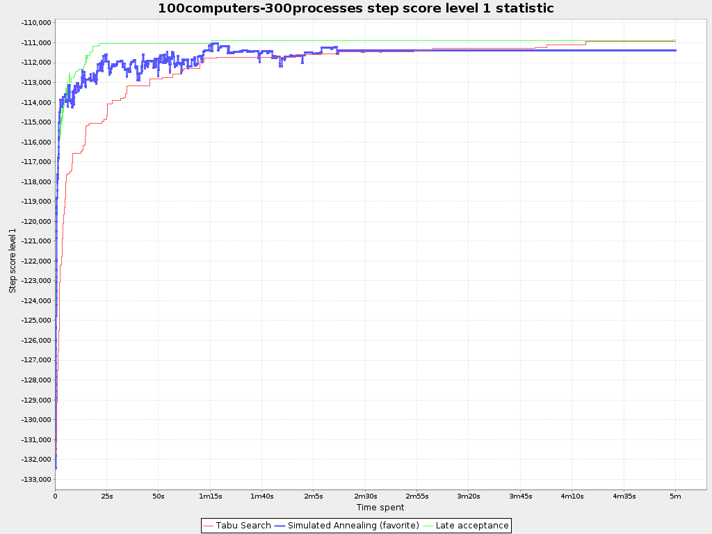
Compare the step score statistic with the best score statistic (especially on parts for which the best score flatlines). If it hits a local optima, the solver should take deteriorating steps to escape it. But it shouldn’t deteriorate too much either.
|
The step score statistic has been seen to slow down the solver noticeably due to GC stress, especially for fast stepping algorithms (such as Simulated Annealing and Late Acceptance). |
17.5.4. Score calculation speed over time statistic (graph and CSV)
To see how fast the scores are calculated, add:
<problemBenchmarks>
...
<problemStatisticType>SCORE_CALCULATION_SPEED</problemStatisticType>
</problemBenchmarks>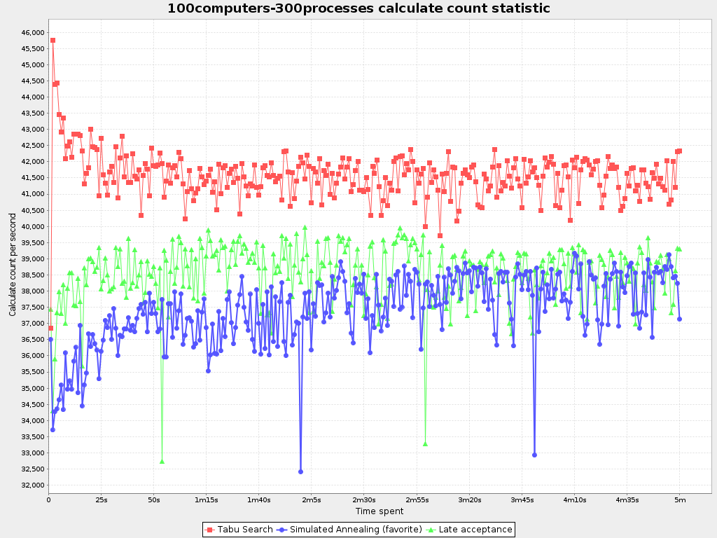
|
The initial high calculation speed is typical during solution initialization: it’s far easier to calculate the score of a solution if only a handful planning entities have been initialized, than when all the planning entities are initialized. After those few seconds of initialization, the calculation speed is relatively stable, apart from an occasional stop-the-world garbage collector disruption. |
17.5.5. Best solution mutation over time statistic (graph and CSV)
To see how much each new best solution differs from the previous best solution, by counting the number of planning variables which have a different value (not including the variables that have changed multiple times but still end up with the same value), add:
<problemBenchmarks>
...
<problemStatisticType>BEST_SOLUTION_MUTATION</problemStatisticType>
</problemBenchmarks>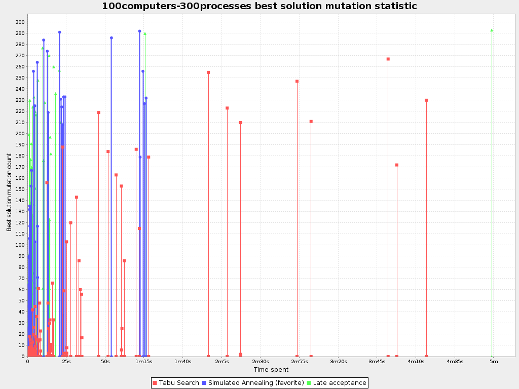
Use Tabu Search - an algorithm that behaves like a human - to get an estimation on how difficult it would be for a human to improve the previous best solution to that new best solution.
17.5.6. Move count per step statistic (graph and CSV)
To see how the selected and accepted move count per step evolves over time, add:
<problemBenchmarks>
...
<problemStatisticType>MOVE_COUNT_PER_STEP</problemStatisticType>
</problemBenchmarks>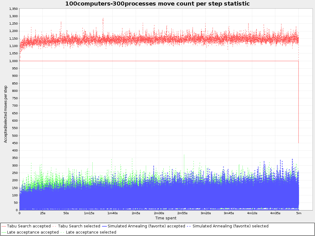
|
This statistic has been seen to slow down the solver noticeably due to GC stress, especially for fast stepping algorithms (such as Simulated Annealing and Late Acceptance). |
17.5.7. Memory use statistic (graph and CSV)
To see how much memory is used, add:
<problemBenchmarks>
...
<problemStatisticType>MEMORY_USE</problemStatisticType>
</problemBenchmarks>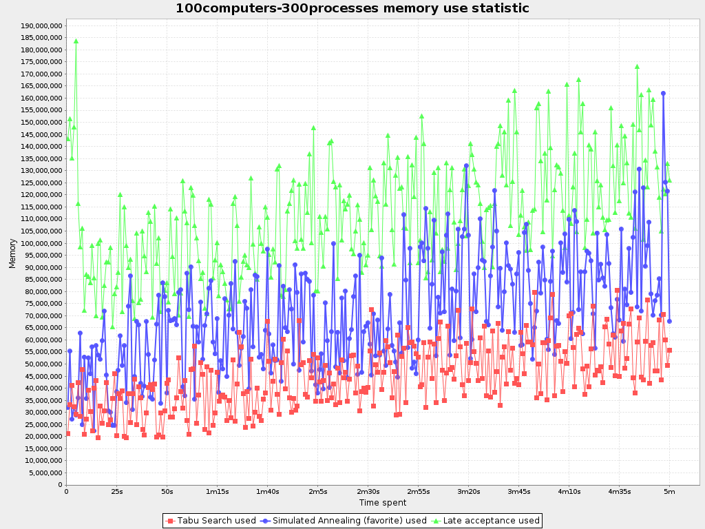
| == The memory use statistic has been seen to affect the solver noticeably. == |
17.6. Statistic per single benchmark (graph and CSV)
17.6.1. Enable a single statistic
A single statistic is static for one dataset for one solver configuration. Unlike a problem statistic, it does not aggregate over solver configurations.
The benchmarker supports outputting single statistics as graphs and CSV (comma separated values) files to the benchmarkDirectory.
To configure one, add a singleStatisticType line:
<plannerBenchmark xmlns="https://www.optaplanner.org/xsd/benchmark" xmlns:xsi="http://www.w3.org/2001/XMLSchema-instance"
xsi:schemaLocation="https://www.optaplanner.org/xsd/benchmark https://www.optaplanner.org/xsd/benchmark/benchmark.xsd">
<benchmarkDirectory>local/data/nqueens/solved</benchmarkDirectory>
<inheritedSolverBenchmark>
<problemBenchmarks>
...
<problemStatisticType>...</problemStatisticType>
<singleStatisticType>PICKED_MOVE_TYPE_BEST_SCORE_DIFF</singleStatisticType>
</problemBenchmarks>
...
</inheritedSolverBenchmark>
...
</plannerBenchmark>Multiple singleStatisticType elements are allowed.
|
These statistic per single benchmark can slow down the solver noticeably, which affects the benchmark results. That’s why they are optional and not enabled by default. |
The following types are supported:
17.6.2. Constraint match total best score over time statistic (graph and CSV)
To see which constraints are matched in the best score (and how much) over time, add:
<problemBenchmarks>
...
<singleStatisticType>CONSTRAINT_MATCH_TOTAL_BEST_SCORE</singleStatisticType>
</problemBenchmarks>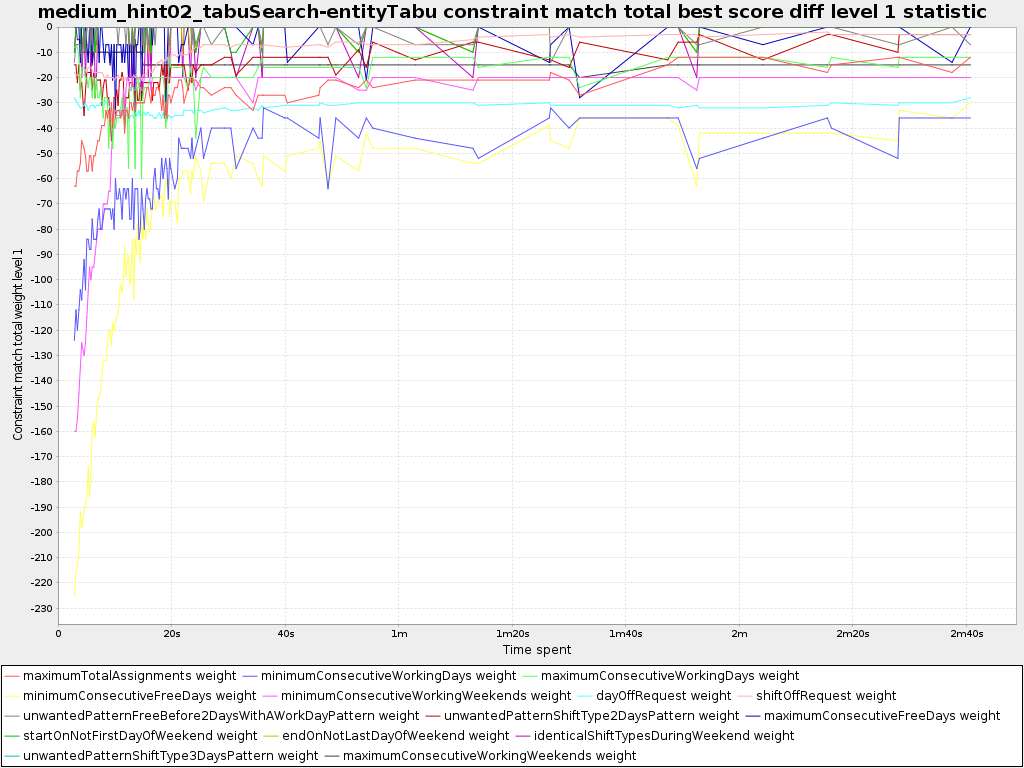
Requires the score calculation to support constraint matches. Constraint Streams and Drools score calculation (Deprecated) support constraint matches automatically, but incremental Java score calculation requires more work.
|
The constraint match total statistics affect the solver noticeably. |
17.6.3. Constraint match total step score over time statistic (graph and CSV)
To see which constraints are matched in the step score (and how much) over time, add:
<problemBenchmarks>
...
<singleStatisticType>CONSTRAINT_MATCH_TOTAL_STEP_SCORE</singleStatisticType>
</problemBenchmarks>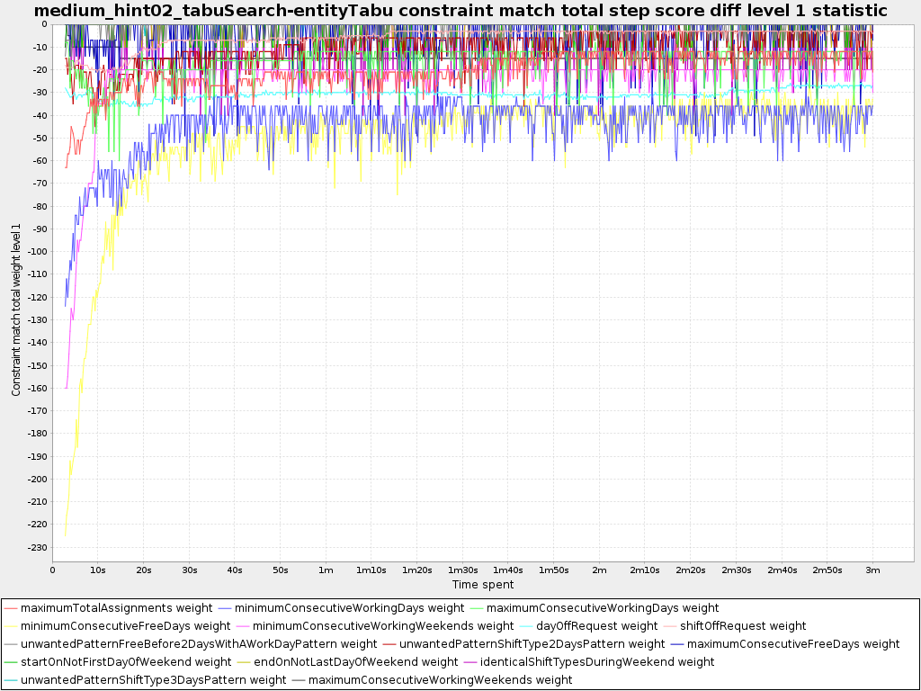
Also requires the score calculation to support constraint matches.
|
The constraint match total statistics affect the solver noticeably. |
17.6.4. Picked move type best score diff over time statistic (graph and CSV)
To see which move types improve the best score (and how much) over time, add:
<problemBenchmarks>
...
<singleStatisticType>PICKED_MOVE_TYPE_BEST_SCORE_DIFF</singleStatisticType>
</problemBenchmarks>
17.6.5. Picked move type step score diff over time statistic (graph and CSV)
To see how much each winning step affects the step score over time, add:
<problemBenchmarks>
...
<singleStatisticType>PICKED_MOVE_TYPE_STEP_SCORE_DIFF</singleStatisticType>
</problemBenchmarks>
17.7. Advanced benchmarking
17.7.1. Benchmarking performance tricks
17.7.1.1. Parallel benchmarking on multiple threads
If you have multiple processors available on your computer, you can run multiple benchmarks in parallel on multiple threads to get your benchmarks results faster:
<plannerBenchmark xmlns="https://www.optaplanner.org/xsd/benchmark" xmlns:xsi="http://www.w3.org/2001/XMLSchema-instance"
xsi:schemaLocation="https://www.optaplanner.org/xsd/benchmark https://www.optaplanner.org/xsd/benchmark/benchmark.xsd">
...
<parallelBenchmarkCount>AUTO</parallelBenchmarkCount>
...
</plannerBenchmark>|
Running too many benchmarks in parallel will affect the results of benchmarks negatively. Leave some processors unused for garbage collection and other processes. |
The following parallelBenchmarkCounts are supported:
-
1(default): Run all benchmarks sequentially. -
AUTO: Let OptaPlanner decide how many benchmarks to run in parallel. This formula is based on experience. It’s recommended to prefer this over the other parallel enabling options. -
Static number: The number of benchmarks to run in parallel.
<parallelBenchmarkCount>2</parallelBenchmarkCount>
|
The |
|
If you have a computer with slow or unreliable cooling, increasing the The |
The benchmarker uses a thread pool internally, but you can optionally plug in a custom ThreadFactory,
for example when running benchmarks on an application server or a cloud platform:
<plannerBenchmark xmlns="https://www.optaplanner.org/xsd/benchmark" xmlns:xsi="http://www.w3.org/2001/XMLSchema-instance"
xsi:schemaLocation="https://www.optaplanner.org/xsd/benchmark https://www.optaplanner.org/xsd/benchmark/benchmark.xsd">
...
<threadFactoryClass>...MyCustomThreadFactory</threadFactoryClass>
...
</plannerBenchmark>|
In the future, we will also support multi-JVM benchmarking. This feature is independent of multithreaded solving or multi-JVM solving. |
17.7.2. Statistical benchmarking
To minimize the influence of your environment and the Random Number Generator on the benchmark results, configure the number of times each single benchmark run is repeated. The results of those runs are statistically aggregated. Each individual result is also visible in the report, as well as plotted in the best score distribution summary.
Just add a <subSingleCount> element to an <inheritedSolverBenchmark> element or in a <solverBenchmark> element:
<?xml version="1.0" encoding="UTF-8"?>
<plannerBenchmark xmlns="https://www.optaplanner.org/xsd/benchmark" xmlns:xsi="http://www.w3.org/2001/XMLSchema-instance"
xsi:schemaLocation="https://www.optaplanner.org/xsd/benchmark https://www.optaplanner.org/xsd/benchmark/benchmark.xsd">
...
<inheritedSolverBenchmark>
...
<solver>
...
</solver>
<subSingleCount>10</subSingleCount>
</inheritedSolverBenchmark>
...
</plannerBenchmark>The subSingleCount defaults to 1 (so no statistical benchmarking).
|
If |
17.7.3. Template-based benchmarking and matrix benchmarking
Matrix benchmarking is benchmarking a combination of value sets.
For example: benchmark four entityTabuSize values (5, 7, 11 and 13) combined with three acceptedCountLimit values (500, 1000 and 2000), resulting in 12 solver configurations.
To reduce the verbosity of such a benchmark configuration, you can use a Freemarker template for the benchmark configuration instead:
<plannerBenchmark xmlns="https://www.optaplanner.org/xsd/benchmark" xmlns:xsi="http://www.w3.org/2001/XMLSchema-instance"
xsi:schemaLocation="https://www.optaplanner.org/xsd/benchmark https://www.optaplanner.org/xsd/benchmark/benchmark.xsd">
...
<inheritedSolverBenchmark>
...
</inheritedSolverBenchmark>
<#list [5, 7, 11, 13] as entityTabuSize>
<#list [500, 1000, 2000] as acceptedCountLimit>
<solverBenchmark>
<name>Tabu Search entityTabuSize ${entityTabuSize} acceptedCountLimit ${acceptedCountLimit}</name>
<solver>
<localSearch>
<unionMoveSelector>
<changeMoveSelector/>
<swapMoveSelector/>
</unionMoveSelector>
<acceptor>
<entityTabuSize>${entityTabuSize}</entityTabuSize>
</acceptor>
<forager>
<acceptedCountLimit>${acceptedCountLimit}</acceptedCountLimit>
</forager>
</localSearch>
</solver>
</solverBenchmark>
</#list>
</#list>
</plannerBenchmark>To configure Matrix Benchmarking for Simulated Annealing (or any other configuration that involves a Score template variable), use the replace() method in the solver benchmark name element:
<plannerBenchmark xmlns="https://www.optaplanner.org/xsd/benchmark" xmlns:xsi="http://www.w3.org/2001/XMLSchema-instance"
xsi:schemaLocation="https://www.optaplanner.org/xsd/benchmark https://www.optaplanner.org/xsd/benchmark/benchmark.xsd">
...
<inheritedSolverBenchmark>
...
</inheritedSolverBenchmark>
<#list ["1hard/10soft", "1hard/20soft", "1hard/50soft", "1hard/70soft"] as startingTemperature>
<solverBenchmark>
<name>Simulated Annealing startingTemperature ${startingTemperature?replace("/", "_")}</name>
<solver>
<localSearch>
<acceptor>
<simulatedAnnealingStartingTemperature>${startingTemperature}</simulatedAnnealingStartingTemperature>
</acceptor>
</localSearch>
</solver>
</solverBenchmark>
</#list>
</plannerBenchmark>|
A solver benchmark name doesn’t allow some characters (such a |
And build it with the class PlannerBenchmarkFactory:
PlannerBenchmarkFactory benchmarkFactory = PlannerBenchmarkFactory.createFromFreemarkerXmlResource(
"org/optaplanner/examples/cloudbalancing/optional/benchmark/cloudBalancingBenchmarkConfigTemplate.xml.ftl");
PlannerBenchmark benchmark = benchmarkFactory.buildPlannerBenchmark();17.7.4. Benchmark report aggregation
The BenchmarkAggregator takes one or more existing benchmarks and merges them into new benchmark report, without actually running the benchmarks again.
This is useful to:
-
Report on the impact of code changes: Run the same benchmark configuration before and after the code changes, then aggregate a report.
-
Report on the impact of dependency upgrades: Run the same benchmark configuration before and after upgrading the dependency, then aggregate a report.
-
Summarize a too verbose report: Select only the interesting solver benchmarks from the existing report. This especially useful on template reports to make the graphs readable.
-
Partially rerun a benchmark: Rerun part of an existing report (for example only the failed or invalid solvers), then recreate the original intended report with the new values.
Compose the aggregated report in the Benchmark aggregator UI:
To display that UI, provide a benchmark config to the BenchmarkAggregatorFrame:
public static void main(String[] args) {
BenchmarkAggregatorFrame.createAndDisplayFromXmlResource(
"org/optaplanner/examples/cloudbalancing/benchmark/cloudBalancingBenchmarkConfig.xml");
}|
Despite that it uses a benchmark configuration as input, it ignores all elements of that configuration,
except for the elements |
In the GUI, select the interesting benchmarks and click the button to generate the aggregated report.
|
All the input reports which are being merged should have been generated with the same OptaPlanner version (excluding hotfix differences) as the |
18. Repeated planning
18.1. Introduction to repeated planning
The problem facts used to create a solution may change before or during the execution of that solution. Delaying planning in order to lower the risk of problem facts changing is not ideal, as an incomplete plan is preferable to no plan.
The following examples demonstrate situations where planning solutions need to be altered due to unpredictable changes:
-
Unforeseen fact changes
-
An employee assigned to a shift calls in sick.
-
An airplane scheduled to take off has a technical delay.
-
One of the machines or vehicles break down.
Unforeseen fact changes benefit from using backup planning.
-
-
Cannot assign all entities immediately
Leave some unassigned. For example:
-
There are 10 shifts at the same time to assign but only nine employees to handle shifts.
For this type of planning, use overconstrained planning.
-
-
Unknown long term future facts
For example:
-
Hospital admissions for the next two weeks are reliable, but those for week three and four are less reliable, and for week five and beyond are not worth planning yet.
This problem benefits from continuous planning.
-
-
Constantly changing problem facts
Use real-time planning.
More CPU time results in a better planning solution.
OptaPlanner allows you to start planning earlier, despite unforeseen changes, as the optimization algorithms support planning a solution that has already been partially planned. This is known as repeated planning.
18.2. Backup planning
Backup planning adds extra score constraints to create space in the planning for when things go wrong. That creates a backup plan within the plan itself.
An example of backup planning is as follows:
-
Create an extra score constraint. For example:
-
Assign an employee as the spare employee (one for every 10 shifts at the same time).
-
Keep one hospital bed open in each department.
-
-
Change the planning problem when an unforeseen event occurs.
For example, if an employee calls in sick:
-
Delete the sick employee and leave their shifts unassigned.
-
Restart the planning, starting from that solution, which now has a different score.
-
The construction heuristics fills in the newly created gaps (probably with the spare employee) and the metaheuristics will improve it even further.
18.3. Overconstrained planning
When there is no feasible solution to assign all planning entities, it is preferable to assign as many entities as possible without breaking hard constraints. This is called overconstrained planning.
By default, OptaPlanner assigns all planning entities, overloads the planning values, and therefore breaks hard constraints. There are two ways to avoid this:
-
Use nullable planning variables, so that some entities are unassigned.
-
Add virtual values to catch the unassigned entities.
18.3.1. Overconstrained planning with nullable variables
If we handle overconstrained planning with nullable variables, the overload entities will be left unassigned:
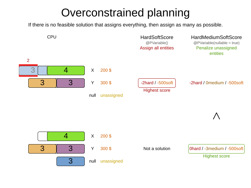
To implement this:
-
Add a score level (usually a medium level between the hard and soft level) by switching
Scoretype. -
Make the planning variable nullable.
-
Add a score constraint on the new level (usually a medium constraint) to penalize the number of unassigned entities (or a weighted sum of them).
18.3.2. Overconstrained planning with virtual values
In overconstrained planning it is often useful to know which resources are lacking. In overconstrained planning with virtual values, the solution indicates which resources to buy.
To implement this:
-
Add an additional score level (usually a medium level between the hard and soft level) by switching
Scoretype. -
Add a number of virtual values. It can be difficult to determine a good formula to calculate that number:
-
Do not add too many, as that will decrease solver efficiency.
-
Importantly, do not add too few as that will lead to an infeasible solution.
-
-
Add a score constraint on the new level (usually a medium constraint) to penalize the number of virtual assigned entities (or a weighted sum of them).
-
Optionally, change all soft constraints to ignore virtual assigned entities.
18.4. Continuous planning (windowed planning)
Continuous planning is the technique of planning one or more upcoming planning periods at the same time and repeating that process monthly, weekly, daily, hourly, or even more frequently. However, as time is infinite, planning all future time periods is impossible.
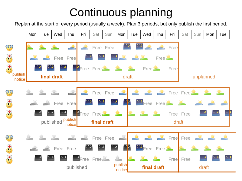
In the employee rostering example above, we re-plan every four days. Each time, we actually plan a window of 12 days, but we only publish the first four days, which is stable enough to share with the employees, so they can plan their social life accordingly.
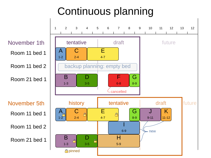
In the hospital bed planning example above, notice the difference between the original planning of November 1st and the new planning of November 5th: some problem facts (F, H, I, J, K) changed in the meantime, which results in unrelated planning entities (G) changing too.
The planning window can be split up in several stages:
-
History
Immutable past time periods. It contains only pinned entities.
-
Recent historic entities can also affect score constraints that apply to movable entities. For example, in nurse rostering, a nurse that has worked the last three historic weekends in a row should not be assigned to three more weekends in a row, because she requires a one free weekend per month.
-
Do not load all historic entities in memory: even though pinned entities do not affect solving performance, they can cause out of memory problems when the data grows to years. Only load those that might still affect the current constraints with a good safety margin.
-
-
Published
Upcoming time periods that have been published. They contain only pinned and/or semi-movable planning entities.
-
The published schedule has been shared with the business. For example, in nurse rostering, the nurses will use this schedule to plan their personal lives, so they require a publish notice of for example 3 weeks in advance. Normal planning will not change that part of schedule.
Changing that schedule later is disruptive, but were exceptions force us to do them anyway (for example someone calls in sick), do change this part of the planning while minimizing disruption with non-disruptive replanning.
-
-
Draft
Upcoming time periods after the published time periods that can change freely. They contain movable planning entities, except for any that are pinned for other reasons (such as being pinned by a user).
-
The first part of the draft, called the final draft, will be published, so these planning entities can change one last time. The publishing frequency, for example once per week, determines the number of time periods that change from draft to published.
-
The latter time periods of the draft are likely change again in later planning efforts, especially if some of the problem facts change by then (for example nurse Ann doesn’t want to work on one of those days).
Despite that these latter planning entities might still change a lot, we can’t leave them out for later, because we would risk painting ourselves into a corner. For example, in employee rostering we could have all our rare skilled employees working the last 5 days of the week that gets published, which won’t reduce the score of that week, but will make it impossible for us to deliver a feasible schedule the next week. So the draft length needs to be longer than the part that will be published first.
-
That draft part is usually not shared with the business yet, because it is too volatile and it would only raise false expectations. However, it is stored in the database and used as a starting point for the next solver.
-
-
Unplanned (out of scope)
Planning entities that are not in the current planning window.
-
If the planning window is too small to plan all entities, you’re dealing with overconstrained planning.
-
If time is a planning variable, the size of the planning window is determined dynamically, in which case the unplanned stage is not applicable.
-
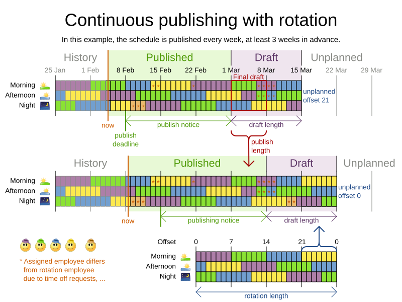
18.4.1. Pinned planning entities
A pinned planning entity doesn’t change during solving. This is commonly used by users to pin down one or more specific assignments and force OptaPlanner to schedule around those fixed assignments.
18.4.1.1. Pin down planning entities with @PlanningPin
To pin some planning entities down, add an @PlanningPin annotation on a boolean getter or field of the planning entity class.
That boolean is true if the entity is pinned down to its current planning values and false otherwise.
-
Add the
@PlanningPinannotation on aboolean:@PlanningEntity public class Lecture { private boolean pinned; ... @PlanningPin public boolean isPinned() { return pinned; } ... }
In the example above, if pinned is true, the lecture will not be assigned to another period or room (even if the current period and rooms fields are null).
18.4.1.2. Configure a PinningFilter
Alternatively, to pin some planning entities down, add a PinningFilter that returns true if an entity is pinned, and false if it is movable.
This is more flexible and more verbose than the @PlanningPin approach.
For example on the nurse rostering example:
-
Add the
PinningFilter:public class ShiftAssignmentPinningFilter implements PinningFilter<NurseRoster, ShiftAssignment> { @Override public boolean accept(NurseRoster nurseRoster, ShiftAssignment shiftAssignment) { ShiftDate shiftDate = shiftAssignment.getShift().getShiftDate(); return nurseRoster.getNurseRosterInfo().isInPlanningWindow(shiftDate); } } -
Configure the
PinningFilter:@PlanningEntity(pinningFilter = ShiftAssignmentPinningFilter.class) public class ShiftAssignment { ... }
18.4.2. Nonvolatile replanning to minimize disruption (semi-movable planning entities)
Replanning an existing plan can be very disruptive. If the plan affects humans (such as employees, drivers, …), very disruptive changes are often undesirable. In such cases, nonvolatile replanning helps by restricting planning freedom: the gain of changing a plan must be higher than the disruption it causes. This is usually implemented by taxing all planning entities that change.
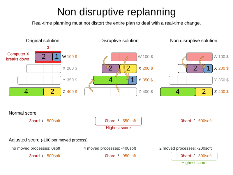
In the machine reassignment example, the entity has both the planning variable machine and its original value originalMachine:
@PlanningEntity(...)
public class ProcessAssignment {
private MrProcess process;
private Machine originalMachine;
private Machine machine;
public Machine getOriginalMachine() {...}
@PlanningVariable(...)
public Machine getMachine() {...}
public boolean isMoved() {
return originalMachine != null && originalMachine != machine;
}
...
}During planning, the planning variable machine changes.
By comparing it with the originalMachine, a change in plan can be penalized:
rule "processMoved"
when
ProcessAssignment(moved == true)
then
scoreHolder.addSoftConstraintMatch(kcontext, -1000);
endThe soft penalty of -1000 means that a better solution is only accepted if it improves the soft score for at least 1000 points per variable changed (or if it improves the hard score).
18.5. Real-time planning
To do real-time planning, combine the following planning techniques:
-
Backup planning - adding extra score constraints to allow for unforeseen changes.
-
Continuous planning - planning for one or more future planning periods.
-
Short planning windows.
This lowers the burden of real-time planning.
As time passes, the problem itself changes. Consider the vehicle routing use case:
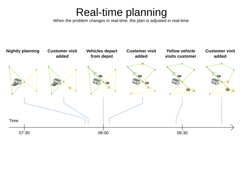
In the example above, three customers are added at different times (07:56, 08:02 and 08:45), after the original customer set finished solving at 07:55, and in some cases, after the vehicles have already left.
OptaPlanner can handle such scenarios with ProblemChange (in combination with pinned planning entities).
18.5.1. ProblemChange
While the Solver is solving, one of the problem facts or planning entities may be changed by an outside event.
For example, an airplane is delayed and needs the runway at a later time.
|
Do not change the problem fact instances used by the |
Add a ProblemChange to the Solver, which it executes in the solver thread as soon as possible.
For example:
public interface Solver<Solution_> {
...
void addProblemChange(ProblemChange<Solution_> problemChange);
boolean isEveryProblemChangeProcessed();
...
}Similarly, you can pass the ProblemChange to the SolverManager:
public interface SolverManager<Solution_, ProblemId_> {
...
CompletableFuture<Void> addProblemChange(ProblemId_ problemId, ProblemChange<Solution_> problemChange);
...
}and the SolverJob:
public interface SolverJob<Solution_, ProblemId_> {
...
CompletableFuture<Void> addProblemChange(ProblemChange<Solution_> problemChange);
...
}Notice the method returns CompletableFuture<Void>, which is completed when a user-defined Consumer accepts
the best solution containing this problem change.
public interface ProblemChange<Solution_> {
void doChange(Solution_ workingSolution, ProblemChangeDirector problemChangeDirector);
}|
The |
To write a ProblemChange correctly, it is important to understand the behavior of a planning clone.
A planning clone of a solution must fulfill these requirements:
-
The clone must represent the same planning problem. Usually it reuses the same instances of the problem facts and problem fact collections as the original.
-
The clone must use different, cloned instances of the entities and entity collections. Changes to an original Solution entity’s variables must not affect its clone.
18.5.1.1. Cloud balancing ProblemChange example
Consider the following example of a ProblemChange implementation in the cloud balancing use case:
public void deleteComputer(final CloudComputer computer) {
solver.addProblemChange((cloudBalance, problemChangeDirector) -> {
CloudComputer workingComputer = problemChangeDirector.lookUpWorkingObject(computer);
if (workingComputer == null) {
throw new IllegalStateException("A computer " + computer + " does not exist. Maybe it has been already deleted.");
}
// First remove the problem fact from all planning entities that use it
for (CloudProcess process : cloudBalance.getProcessList()) {
if (process.getComputer() == workingComputer) {
problemChangeDirector.changeVariable(process, "computer",
workingProcess -> workingProcess.setComputer(null));
}
}
// A SolutionCloner does not clone problem fact lists (such as computerList)
// Shallow clone the computerList so only workingSolution is affected, not bestSolution or guiSolution
ArrayList<CloudComputer> computerList = new ArrayList<>(cloudBalance.getComputerList());
cloudBalance.setComputerList(computerList);
// Remove the problem fact itself
problemChangeDirector.removeProblemFact(workingComputer, computerList::remove);
});
}-
Any change in a
ProblemChangemust be done on the@PlanningSolutioninstance ofscoreDirector.getWorkingSolution(). -
The
workingSolutionis a planning clone of theBestSolutionChangedEvent'sbestSolution.-
The
workingSolutionin theSolveris never the same solution instance as in the rest of your application: it is a planning clone. -
A planning clone also clones the planning entities and planning entity collections.
Thus, any change on the planning entities must happen on the
workingSolutioninstance passed to theProblemChange.doChange(Solution_ workingSolution, ProblemChangeDirector problemChangeDirector)method.
-
-
Use the method
ProblemChangeDirector.lookUpWorkingObject()to translate and retrieve the working solution’s instance of an object. This requires annotating a property of that class as the @PlanningId. -
A planning clone does not clone the problem facts, nor the problem fact collections. Therefore the
workingSolutionand thebestSolutionshare the same problem fact instances and the same problem fact list instances.Any problem fact or problem fact list changed by a
ProblemChangemust be problem cloned first (which can imply rerouting references in other problem facts and planning entities). Otherwise, if theworkingSolutionandbestSolutionare used in different threads (for example a solver thread and a GUI event thread), a race condition can occur.
18.5.1.2. Cloning solutions to avoid race conditions in real-time planning
Many types of changes can leave a planning entity uninitialized, resulting in a partially initialized solution. This is acceptable, provided the first solver phase can handle it.
All construction heuristics solver phases can handle a partially initialized solution, so it is recommended to configure such a solver phase as the first phase.
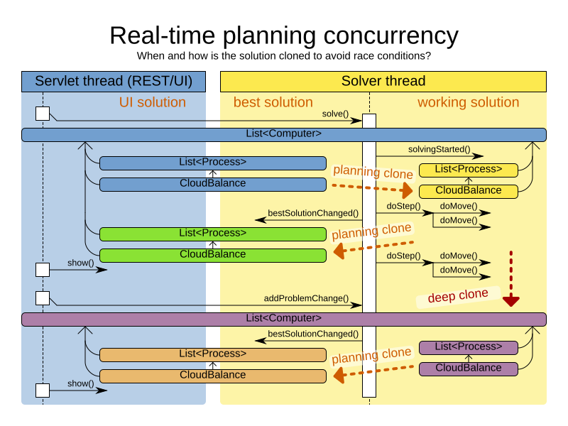
The process occurs as follows:
-
The
Solverstops. -
Runs the
ProblemChange. -
restarts.
This is a warm start because its initial solution is the adjusted best solution of the previous run.
-
Each solver phase runs again.
This implies the construction heuristic runs again, but because little or no planning variables are uninitialized (unless you have a nullable planning variable), it finishes much quicker than in a cold start.
-
Each configured
Terminationresets (both in solver and phase configuration), but a previous call toterminateEarly()is not undone.Terminationis not usually configured (except in daemon mode); instead,Solver.terminateEarly()is called when the results are needed. Alternatively, configure aTerminationand use the daemon mode in combination withBestSolutionChangedEventas described in the following section.
18.5.2. Daemon: solve() does not return
In real-time planning, it is often useful to have a solver thread wait when it runs out of work, and immediately resume solving a problem once new problem fact changes are added.
Putting the Solver in daemon mode has the following effects:
-
If the
Solver'sTerminationterminates, it does not return fromsolve(), but blocks its thread instead (which frees up CPU power).-
Except for
terminateEarly(), which does make it return fromsolve(), freeing up system resources and allowing an application to shutdown gracefully. -
If a
Solverstarts with an empty planning entity collection, it waits in the blocked state immediately.
-
-
If a
ProblemChangeis added, it goes into the running state, applies theProblemChangeand runs theSolveragain.
To use the Solver in daemon mode:
-
Enable
daemonmode on theSolver:<solver xmlns="https://www.optaplanner.org/xsd/solver" xmlns:xsi="http://www.w3.org/2001/XMLSchema-instance" xsi:schemaLocation="https://www.optaplanner.org/xsd/solver https://www.optaplanner.org/xsd/solver/solver.xsd"> <daemon>true</daemon> ... </solver>Do not forget to call
Solver.terminateEarly()when your application needs to shutdown to avoid killing the solver thread unnaturally. -
Subscribe to the
BestSolutionChangedEventto process new best solutions found by the solver thread.A
BestSolutionChangedEventdoes not guarantee that everyProblemChangehas been processed already, nor that the solution is initialized and feasible. -
To ignore
BestSolutionChangedEvents with such invalid solutions, do the following:public void bestSolutionChanged(BestSolutionChangedEvent<CloudBalance> event) { if (event.isEveryProblemChangeProcessed() // Ignore infeasible (including uninitialized) solutions && event.getNewBestSolution().getScore().isFeasible()) { ... } } -
Use
Score.isSolutionInitialized()instead ofScore.isFeasible()to only ignore uninitialized solutions, but do accept infeasible solutions too.
18.6. Multi-stage planning
In multi-stage planning, complex planning problems are broken down in multiple stages. A typical example is train scheduling, where one department decides where and when a train will arrive or depart and another department assigns the operators to the actual train cars or locomotives.
Each stage has its own solver configuration (and therefore its own SolverFactory):
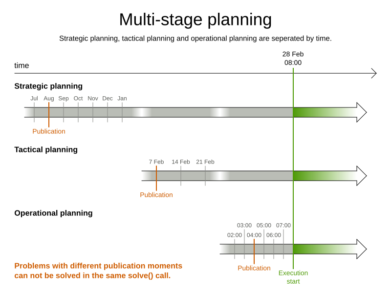
Planning problems with different publication deadlines must use multi-stage planning. But problems with the same publication deadline, solved by different organizational groups are also initially better off with multi-stage planning, because of Conway’s law and the high risk associated with unifying such groups.
Similarly to Partitioned Search, multi-stage planning leads to suboptimal results. Nevertheless, it might be beneficial in order to simplify the maintenance, ownership, and help to start a project.
Do not confuse multi-stage planning with multi-phase solving.
19. Integration
19.1. Overview
OptaPlanner’s input and output data (the planning problem and the best solution) are plain old JavaBeans (POJOs), so integration with other Java technologies is straightforward. For example:
-
To read a planning problem from the database (and store the best solution in it), annotate the domain POJOs with JPA annotations.
-
To read a planning problem from an XML file (and store the best solution in it), annotate the domain POJOs with JAXB annotations.
-
To expose the Solver as a REST Service that reads the planning problem and responds with the best solution, annotate the domain POJOs with JAXB or Jackson annotations and hook the
Solverin Camel or RESTEasy.
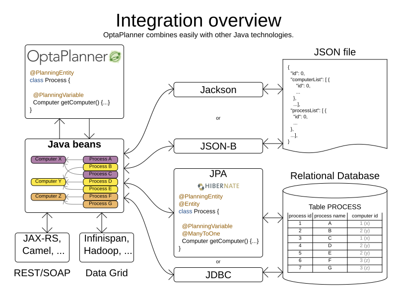
19.2. Persistent storage
19.2.1. Database: JPA and Hibernate
Enrich domain POJOs (solution, entities and problem facts) with JPA annotations
to store them in a database by calling EntityManager.persist().
|
Do not confuse JPA’s |
19.2.1.1. JPA and Hibernate: persisting a Score
The optaplanner-persistence-jpa jar provides a JPA score converter for every built-in score type.
@PlanningSolution
@Entity
public class CloudBalance {
@PlanningScore
@Convert(converter = HardSoftScoreConverter.class)
protected HardSoftScore score;
...
}Please note that the converters make JPA and Hibernate serialize the score in a single VARCHAR column.
This has the disadvantage that the score cannot be used in a SQL or JPA-QL query to efficiently filter the results, for example to query all infeasible schedules.
To avoid this limitation, implement the CompositeUserType to persist each score level into a separate database table column.
19.2.1.2. JPA and Hibernate: planning cloning
In JPA and Hibernate, there is usually a @ManyToOne relationship from most problem fact classes to the planning solution class.
Therefore, the problem fact classes reference the planning solution class, which implies that when the solution is planning cloned, they need to be cloned too.
Use an @DeepPlanningClone on each such problem fact class to enforce that:
@PlanningSolution // OptaPlanner annotation
@Entity // JPA annotation
public class Conference {
@OneToMany(mappedBy="conference")
private List<Room> roomList;
...
}@DeepPlanningClone // OptaPlanner annotation: Force the default planning cloner to planning clone this class too
@Entity // JPA annotation
public class Room {
@ManyToOne
private Conference conference; // Because of this reference, this problem fact needs to be planning cloned too
}Neglecting to do this can lead to persisting duplicate solutions, JPA exceptions or other side effects.
19.2.2. XML or JSON: JAXB
Enrich domain POJOs (solution, entities and problem facts) with JAXB annotations to serialize them to/from XML or JSON.
Add a dependency to the optaplanner-persistence-jaxb jar to take advantage of these extra integration features:
19.2.2.1. JAXB: marshalling a Score
When a Score is marshalled to XML or JSON by the default JAXB configuration, it’s corrupted.
To fix that, configure the appropriate ScoreJaxbAdapter:
@PlanningSolution
@XmlRootElement @XmlAccessorType(XmlAccessType.FIELD)
public class CloudBalance {
@PlanningScore
@XmlJavaTypeAdapter(HardSoftScoreJaxbAdapter.class)
private HardSoftScore score;
...
}For example, this generates pretty XML:
<cloudBalance>
...
<score>0hard/-200soft</score>
</cloudBalance>The same applies for a bendable score:
@PlanningSolution
@XmlRootElement @XmlAccessorType(XmlAccessType.FIELD)
public class Schedule {
@PlanningScore
@XmlJavaTypeAdapter(BendableScoreJaxbAdapter.class)
private BendableScore score;
...
}For example, with a hardLevelsSize of 2 and a softLevelsSize of 3, that will generate:
<schedule>
...
<score>[0/0]hard/[-100/-20/-3]soft</score>
</schedule>The hardLevelsSize and softLevelsSize implied, when reading a bendable score from an XML element, must always be in sync with those in the solver.
19.2.3. JSON: Jackson
Enrich domain POJOs (solution, entities and problem facts) with Jackson annotations to serialize them to/from JSON.
Add a dependency to the optaplanner-persistence-jackson jar and register OptaPlannerJacksonModule:
ObjectMapper objectMapper = new ObjectMapper();
objectMapper.registerModule(OptaPlannerJacksonModule.createModule());19.2.3.1. Jackson: marshalling a Score
When a Score is marshalled to/from JSON by the default Jackson configuration, it fails.
The OptaPlannerJacksonModule fixes that, by using HardSoftScoreJacksonSerializer,
HardSoftScoreJacksonDeserializer, etc.
@PlanningSolution
public class CloudBalance {
    @PlanningScore
    private HardSoftScore score;
...
}For example, this generates:
{
"score":"0hard/-200soft"
...
}|
When reading a This JSON implies the |
When a field is the Score supertype (instead of a specific type such as HardSoftScore), it uses PolymorphicScoreJacksonSerializer and PolymorphicScoreJacksonDeserializer
to record the score type in JSON too, otherwise it would be impossible to deserialize it:
@PlanningSolution
public class CloudBalance {
@PlanningScore
private Score score;
...
}For example, this generates:
{
"score":{"HardSoftScore":"0hard/-200soft"}
...
}19.2.4. JSON: JSON-B
Enrich domain POJOs (solution, entities and problem facts) with JSON-B annotations to serialize them to/from JSON.
Add a dependency to the optaplanner-persistence-jsonb jar and use OptaPlannerJsonbConfig to create a Jsonb instance:
JsonbConfig config = OptaPlannerJsonbConfig.createConfig();
Jsonb jsonb = JsonbBuilder.create(config);19.2.4.1. JSON-B: marshalling a Score
When a Score is marshalled to/from JSON by the default JSON-B configuration, it fails.
The OptaPlannerJsonbConfig fixes that, by using adapters including BendableScoreJsonbAdapter, HardSoftScoreJsonbAdapter, etc.
@PlanningSolution
public class CloudBalance {
@PlanningScore
private HardSoftScore score;
...
}For example, this generates:
{"hardSoftScore":"0hard/-200soft"}The same applies for a bendable score:
@PlanningSolution
public class CloudBalance {
@PlanningScore
private BendableScore score;
...
}This generates:
{"bendableScore":"[0/0]hard/[-200/-20/0]soft"}19.3. Quarkus
To use OptaPlanner with Quarkus, read the Quarkus Java quick start. If you are starting a new project, visit the code.quarkus.io and select the OptaPlanner AI constraint solver extension before generating your application.
|
Drools score calculation is incompatible with the |
Following properties are supported in the Quarkus application.properties:
- quarkus.optaplanner.solver-manager.parallel-solver-count
-
The number of solvers that run in parallel. This directly influences CPU consumption. Defaults to
AUTO. - quarkus.optaplanner.solver-config-xml
-
A classpath resource to read the solver configuration XML. Defaults to
solverConfig.xml. If this property isn’t specified, that file is optional. - quarkus.optaplanner.score-drl (deprecated)
-
A classpath resource to read the score DRL. Defaults to
constraints.drl. Do not define this property when aConstraintProvider,EasyScoreCalculatororIncrementalScoreCalculatorclass exists. - quarkus.optaplanner.solver.environment-mode
-
Enable runtime assertions to detect common bugs in your implementation during development.
- quarkus.optaplanner.solver.daemon
-
Enable daemon mode. In daemon mode, non-early termination pauses the solver instead of stopping it, until the next problem fact change arrives. This is often useful for real-time planning. Defaults to
false. - quarkus.optaplanner.solver.move-thread-count
-
Enable multithreaded solving for a single problem, which increases CPU consumption. Defaults to
NONE. See multithreaded incremental solving. - quarkus.optaplanner.solver.domain-access-type
-
How OptaPlanner should access the domain model. See the domain access section for more details. Defaults to
GIZMO. The other possible value isREFLECTION. - quarkus.optaplanner.solver.constraint-stream-impl-type
-
What Constraint Stream implementation to use. See the variant implementation types section for more details. Defaults to
DROOLS. The other possible value isBAVET. - quarkus.optaplanner.solver.termination.spent-limit
-
How long the solver can run. For example:
30sis 30 seconds.5mis 5 minutes.2his 2 hours.1dis 1 day. - quarkus.optaplanner.solver.termination.unimproved-spent-limit
-
How long the solver can run without finding a new best solution after finding a new best solution. For example:
30sis 30 seconds.5mis 5 minutes.2his 2 hours.1dis 1 day. - quarkus.optaplanner.solver.termination.best-score-limit
-
Terminates the solver when a specific or higher score has been reached. For example:
0hard/-1000softterminates when the best score changes from0hard/-1200softto0hard/-900soft. Wildcards are supported to replace numbers. For example:0hard/*softto terminate when any feasible score is reached. - quarkus.optaplanner.benchmark.solver-benchmark-config-xml
-
A classpath resource to read the benchmark configuration XML. Defaults to solverBenchmarkConfig.xml. If this property isn’t specified, that solverBenchmarkConfig.xml is optional.
- quarkus.optaplanner.benchmark.result-directory
-
Where the benchmark results are written to. Defaults to target/benchmarks.
- quarkus.optaplanner.benchmark.solver.termination.spent-limit
-
How long solver should be run in a benchmark run. For example:
30sis 30 seconds.5mis 5 minutes.2his 2 hours.1dis 1 day. Also supports ISO-8601 format, see Duration.
19.4. Spring Boot
To use OptaPlanner on Spring Boot, add the optaplanner-spring-boot-starter dependency
and read the Spring Boot Java quick start.
|
Drools score calculation is currently incompatible with the dependency |
These properties are supported in Spring’s application.properties:
- optaplanner.solver-manager.parallel-solver-count
-
The number of solvers that run in parallel. This directly influences CPU consumption. Defaults to
AUTO. - optaplanner.solver-config-xml
-
A classpath resource to read the solver configuration XML. Defaults to
solverConfig.xml. If this property isn’t specified, that file is optional. - optaplanner.score-drl (deprecated)
-
A classpath resource to read the score DRL. Defaults to
constraints.drl. Do not define this property when aConstraintProvider,EasyScoreCalculatororIncrementalScoreCalculatorclass exists. - optaplanner.solver.environment-mode
-
Enable runtime assertions to detect common bugs in your implementation during development.
- optaplanner.solver.daemon
-
Enable daemon mode. In daemon mode, non-early termination pauses the solver instead of stopping it, until the next problem fact change arrives. This is often useful for real-time planning. Defaults to
false. - optaplanner.solver.move-thread-count
-
Enable multithreaded solving for a single problem, which increases CPU consumption. Defaults to
NONE. See multithreaded incremental solving. - optaplanner.solver.domain-access-type
-
How OptaPlanner should access the domain model. See the domain access section for more details. Defaults to
REFLECTION. The other possible value isGIZMO. - optaplanner.solver.constraint-stream-impl-type
-
What Constraint Stream implementation to use. See the variant implementation types section for more details. Defaults to
DROOLS. The other possible value isBAVET. - optaplanner.solver.termination.spent-limit
-
How long the solver can run. For example:
30sis 30 seconds.5mis 5 minutes.2his 2 hours.1dis 1 day. - optaplanner.solver.termination.unimproved-spent-limit
-
How long the solver can run without finding a new best solution after finding a new best solution. For example:
30sis 30 seconds.5mis 5 minutes.2his 2 hours.1dis 1 day. - optaplanner.solver.termination.best-score-limit
-
Terminates the solver when a specific or higher score has been reached. For example:
0hard/-1000softterminates when the best score changes from0hard/-1200softto0hard/-900soft. Wildcards are supported to replace numbers. For example:0hard/*softto terminate when any feasible score is reached. - optaplanner.benchmark.solver-benchmark-config-xml
-
A classpath resource to read the benchmark configuration XML. Defaults to solverBenchmarkConfig.xml. If this property isn’t specified, that solverBenchmarkConfig.xml is optional.
- optaplanner.benchmark.result-directory
-
Where the benchmark results are written to. Defaults to target/benchmarks.
- optaplanner.benchmark.solver.termination.spent-limit
-
How long solver should be run in a benchmark run. For example:
30sis 30 seconds.5mis 5 minutes.2his 2 hours.1dis 1 day. Also supports ISO-8601 format, see Duration.
19.5. SOA and ESB
19.5.1. Camel and Karaf
Camel is an enterprise integration framework which includes support for OptaPlanner (starting from Camel 2.13). It can expose a use case as a REST service, a SOAP service, a JMS service, …
Read the documentation for the camel-optaplanner component. That component works in Karaf too.
19.6. Other environments
19.6.1. Java platform module system (Jigsaw)
When using OptaPlanner from code on the modulepath (Java 9 and higher),
open your packages that contain your domain objects, constraints and solver configuration
to all modules in your module-info.java file:
module org.optaplanner.cloudbalancing {
requires org.optaplanner.core;
...
opens org.optaplanner.examples.cloudbalancing; // Solver configuration
opens org.optaplanner.examples.cloudbalancing.domain; // Domain classes
opens org.optaplanner.examples.cloudbalancing.score; // Constraints
...
}Otherwise OptaPlanner can’t reach those classes or files, even if they are exported.
19.6.2. OSGi
Integration with OSGi is not supported.
19.6.3. Android
Android is not a complete JVM (because some JDK libraries are missing), but OptaPlanner works on Android with easy Java or incremental Java score calculation. The Drools rule engine does not work on Android yet, so Constraint Streams and Drools score calculation (Deprecated) doesn’t work on Android and its dependencies need to be excluded.
Workaround to use OptaPlanner on Android:
-
Add a dependency to the
build.gradlefile in your Android project to exclude OptaPlanner’soptaplanner-constraint-streams-droolsandoptaplanner-constraint-drlmodules:dependencies { ... implementation('org.optaplanner:optaplanner-core:...') { exclude group: 'org.optaplanner', module: 'optaplanner-constraint-streams-drools' exclude group: 'org.optaplanner', module: 'optaplanner-constraint-drl' } ... }
19.7. Integration with human planners (politics)
A good OptaPlanner implementation beats any good human planner for non-trivial datasets. Many human planners fail to accept this, often because they feel threatened by an automated system.
But despite that, both can benefit if the human planner becomes the supervisor of OptaPlanner:
-
The human planner defines, validates and tweaks the score function.
-
The human planner tweaks the constraint weights of the constraint configuration in a UI, as the business priorities change over time.
-
When the business changes, the score function often needs to change too. The human planner can notify the developers to add, change or remove score constraints.
-
-
The human planner is always in control of OptaPlanner.
-
As shown in the course scheduling example, the human planner can pin down one or more planning variables to a specific planning value. Because they are pinned, OptaPlanner does not change them: it optimizes the planning around the enforcements made by the human. If the human planner pins down all planning variables, he/she sidelines OptaPlanner completely.
-
In a prototype implementation, the human planner occasionally uses pinning to intervene, but as the implementation matures, this should become obsolete. The feature should be kept available as a reassurance for the humans, and in the event that the business changes dramatically before the score constraints are adjusted accordingly.
-
For this reason, it is recommended that the human planner is actively involved in your project.
19.8. Sizing hardware and software
Before sizing a OptaPlanner service, first understand the typical behaviour of a Solver.solve() call:
Understand these guidelines to decide the hardware for a OptaPlanner service:
-
RAM memory: Provision plenty, but no need to provide more.
-
The problem dataset, loaded before OptaPlanner is called, often consumes the most memory. It depends on the problem scale.
-
For example, in the Machine Reassignment example some datasets use over 1GB in memory. But in most examples, they use just a few MB.
-
If this is a problem, review the domain class structure: remove classes or fields that OptaPlanner doesn’t need during solving.
-
OptaPlanner usually has up to three solution instances: the internal working solution, the best solution and the old best solution (when it’s being replaced). However, these are all a planning clone of each other, so many problem fact instances are shared between those solution instances.
-
-
During solving, the memory is very volatile, because solving creates many short-lived objects. The Garbage Collector deletes these in bulk and therefore needs some heap space as a buffer.
-
The maximum size of the JVM heap space can be in three states:
-
Insufficient: An
OutOfMemoryExceptionis thrown (often because the Garbage Collector is using more than 98% of the CPU time). -
Narrow: The heap buffer for those short-lived instances is too small, therefore the Garbage Collector needs to run more than it would like to, which causes a performance loss.
-
Profiling shows that in the heap chart, the used heap space frequently touches the max heap space during solving. It also shows that the Garbage Collector has a significant CPU usage impact.
-
Adding more heap space increases the score calculation speed.
-
-
Plenty: There is enough heap space. The Garbage Collector is active, but its CPU usage is low.
-
Adding more heap space does not increase performance.
-
Usually, this is around 300 to 500MB above the dataset size, regardless of the problem scale (except with nearby selection and caching move selector, neither are used by default).
-
-
-
-
CPU power: More is better.
-
Improving CPU speed directly increases the score calculation speed.
-
If the CPU power is twice as fast, it takes half the time to find the same result. However, this does not guarantee that it finds a better result in the same time, nor that it finds a similar result for a problem twice as big in the same time.
-
Increasing CPU power usually does not resolve scaling issues, because planning problems scale exponentially. Power tweaking the solver configuration has far better results for scaling issues than throwing hardware at it.
-
-
During the
solve()method, the CPU power will max out until it returns (except in daemon mode or if your SolverEventListener writes the best solution to disk or the network).
-
-
Number of CPU cores: one CPU core per active Solver, plus at least one one for the operating system.
-
So in a multitenant application, which has one Solver per tenant, this means one CPU core per tenant, unless the number of solver threads is limited, as that limits the number of tenants being solved in parallel.
-
With Partitioned Search, presume one CPU core per partition (per active tenant), unless the number of partition threads is limited.
-
To reduce the number of used cores, it can be better to reduce the partition threads (so solve some partitions sequentially) than to reduce the number of partitions.
-
-
In use cases with many tenants (such as scheduling Software as a Service) or many partitions, it might not be affordable to provision that many CPUs.
-
Reduce the number of active Solvers at a time. For example: give each tenant only one minute of machine time and use a
ExecutorServicewith a fixed thread pool to queue requests. -
Distribute the Solver runs across the day (or night). This is especially an opportunity in SaaS that’s used across the globe, due to timezones: UK and India can use the same CPU core when scheduling at night.
-
-
The SolverManager will take care of the orchestration, especially in those underfunded environments in which solvers (and partitions) are forced to share CPU cores or wait in line.
-
-
I/O (network, disk, …): Not used during solving.
-
OptaPlanner is not a web server: a solver thread does not block (unlike a servlet thread), each one fully drains a CPU.
-
A web server can handle 24 active servlets threads with eight cores without performance loss, because most servlets threads are blocking on I/O.
-
However, 24 active solver threads with eight cores will cause each solver’s score calculation speed to be three times slower, causing a big performance loss.
-
-
Note that calling any I/O during solving, for example a remote service in your score calculation, causes a huge performance loss because it’s called thousands of times per second, so it should complete in microseconds. So no good implementation does that.
-
Keep these guidelines in mind when selecting and configuring the software. See our blog archive for the details of our experiments, which use our diverse set of examples. Your mileage may vary.
-
Operating System
-
No experimentally proven advice yet (but prefer Linux anyway).
-
-
JDK
-
Version: Our benchmarks have consistently shown improvements in performance when comparing new JDK releases with their predecessors. It is therefore recommended using the latest available JDK. If you’re interested in the performance comparisons of OptaPlanner running of different JDK releases, you can find them in the form of blog posts in our blog archive.
-
Garbage Collector: ParallelGC can be potentially between 5% and 35% faster than G1GC (the default). Unlike web servers, OptaPlanner needs a GC focused on throughput, not latency. Use
-XX:+UseParallelGCto turn on ParallelGC.
-
-
Logging can have a severe impact on performance.
-
Debug logging
org.droolscan reduce performance by a factor of 7. -
Debug logging
org.optaplannercan be between 0% and 15% slower than info logging. Trace logging can be between 5% and 70% slower than info logging. -
Synchronous logging to a file has an additional significant impact for debug and trace logging (but not for info logging).
-
-
Avoid a cloud environment in which you share your CPU core(s) with other virtual machines or containers. Performance (and therefore solution quality) can be unreliable when the available CPU power varies greatly.
Keep in mind that the perfect hardware/software environment will probably not solve scaling issues (even Moore’s law is too slow). There is no need to follow these guidelines to the letter.
20. Design patterns
20.1. Design patterns introduction
OptaPlanner design patterns are generic reusable solutions to common challenges in the model or architecture of projects that perform constraint solving. The design patterns in this section list and solve common design challenges.
20.2. Domain modeling guidelines
Follow the guidelines listed in this section to create a well thought-out model that can contribute significantly to the success of your planning.
-
Draw a class diagram of your domain model.
-
Make sure there are no duplications in your data model and that relationships between objects are clearly defined.
-
Create sample instances for each class. For example, in the employee rostering
Employeeclass, createAnn,Bert, andCarl.
-
-
Determine which relationships (or fields) change during planning and color them orange. One side of these relationships will become a planning variable later on. For example, in employee rostering, the
ShifttoEmployeerelationship changes during planning, so it is orange. However, other relationships, such as fromEmployeetoSkill, are immutable during planning because OptaPlanner cannot assign an extra skill to an employee. -
If there are multiple relationships (or fields), check for shadow variables. A shadow variable changes during planning, but its value can be calculated based on one or more genuine planning variables, without dispute. Color shadow relationships (or fields) purple.
Only one side of a bi-directional relationship can be a genuine planning variable. The other side will become an inverse relation shadow variable later on. Keep bi-directional relationships orange.
-
If the goal is to find an optimal order of elements, use the Chained Through Time pattern.
-
If there is an orange many-to-many relationship, replace it with a one-to-many and a many-to-one relationship to a new intermediate class.
OptaPlanner does not currently support a
@PlanningVariableannotation on a collection.For example, in the Employee Rostering starter application the
ShiftAssignmentclass is the many-to-many relationship betweenShiftandEmployee.Shiftcontains every shift time that needs to be filled with an employee.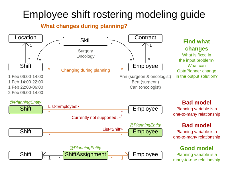
-
Annotate a many-to-one relationship with a
@PlanningEntityannotation. Usually the many side of the relationship is the planning entity class that contains the planning variable. If the relationship is bi-directional, both sides are a planning entity class but usually the many side has the planning variable and the one side has the shadow variable. For example, in employee rostering, theShiftAssignmentclass has an@PlanningEntityannotation. -
Make sure that the planning entity class has at least one problem property. A planning entity class cannot consist of only planning variables or an ID and only planning variables.
-
Remove any surplus
@PlanningVariableannotations so that they become problem properties. Doing this significantly decreases the search space size and significantly increases solving efficiency. For example, in employee rostering, theShiftAssignmentclass should not annotate both theShiftandEmployeerelationship with@PlanningVariable. -
Make sure that when all planning variables have a value of
null, the planning entity instance is describable to the business people. Planning variables have a value ofnullwhen the planning solution is uninitialized.-
A surrogate ID does not suffice as the required minimum of one problem property.
-
There is no need to add a hard constraint to assure that two planning entities are different. They are already different due to their problem properties.
-
In some cases, multiple planning entity instances have the same set of problem properties. In such cases, it can be useful to create an extra problem property to distinguish them. For example, in employee rostering, the
ShiftAssignmentclass has the problem propertyShiftas well as the problem propertyindexInShiftwhich is anintclass.
-
-
-
Choose the model in which the number of planning entities is fixed during planning. For example, in the employee rostering, it is impossible to know in advance how many shifts each employee will have before OptaPlanner solves the model and the results can differ for each solution found. On the other hand, the number of employees per shift is known in advance, so it is better to make the
Shiftrelationship a problem property and theEmployeerelationship a planning variable as shown in the following examples.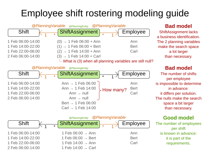
In the following diagram, each row is a different example and shows the relationship in that example’s data model. For the N Queens example, the Queen entity has a Row planning variable, which stores objects of type row. Many Queens may point to one Row.
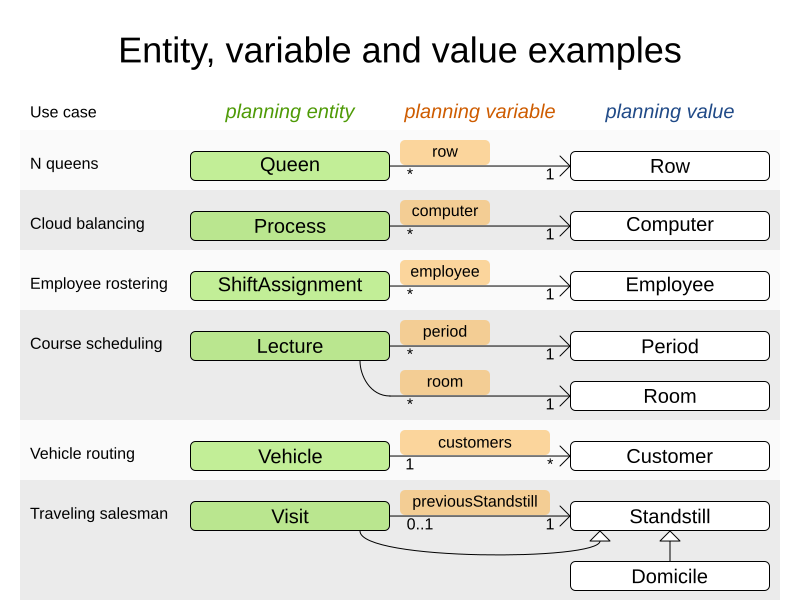
|
Course scheduling is different because it uses two planning variables. Vehicle routing is different because it uses a planning list variable. Traveling salesman is different because it uses a chained planning variable. |
20.3. Assigning time to planning entities
Dealing with time and dates in planning problems may be problematic because it is dependent on the needs of your use case.
There are several representations of timestamps, dates, durations and periods in Java. Choose the right representation type for your use case:
-
java.util.Date(deprecated): a slow, error-prone way to represent timestamps. Do not use. -
java.time.LocalDateTime,LocalDate,DayOfWeek,Duration,Period, …: an accurate way to represent and calculate with timestamps, dates, …-
Supports timezones and DST (Daylight Saving Time).
-
Requires Java 8 or higher.
-
-
intorlong: Caches a timestamp as a simplified number of coarse-grained time units (such as minutes) from the start of the global planning time window or the epoch.-
For example: a
LocalDateTimeof1-JAN 08:00:00becomes anintof400minutes. Similarly1-JAN 09:00:00becomes460minutes. -
It often represents an extra field in a class, alongside the
LocalDateTimefield from which it was calculated. TheLocalDateTimeis used for user visualization, but theintis used in the score constraints. -
It is faster in calculations, which is especially useful in the TimeGrain pattern.
-
Do not use if timezones or DST affect the score constraints.
-
There are also several designs for assigning a planning entity to a starting time (or date):
-
If the starting time is fixed beforehand, it is not a planning variable (in that solver).
-
For example, in the hospital bed planning example, the arrival day of each patient is fixed beforehand.
-
This is common in multi-stage planning, when the starting time has been decided already in an earlier planning stage.
-
-
If the starting time is not fixed, it is a planning variable (genuine or shadow).
-
If all planning entities have the same duration, use the Timeslot pattern.
-
For example in course scheduling, all lectures take one hour. Therefore, each timeslot is one hour.
-
Even if the planning entities have different durations, but the same duration per type, it’s often appropriate.
-
For example in conference scheduling, breakout talks take one hour and lab talks take 2 hours. But there’s an enumeration of the timeslots and each timeslot only accepts one talk type.
-
-
-
If the duration differs and time is rounded to a specific time granularity (for example 5 minutes) use the TimeGrain pattern.
-
For example in meeting scheduling, all meetings start at 15 minute intervals. All meetings take 15, 30, 45, 60, 90 or 120 minutes.
-
-
If the duration differs and one task starts immediately after the previous task (assigned to the same executor) finishes, use the Chained Through Time pattern.
-
For example in time windowed vehicle routing, each vehicle departs immediately to the next customer when the delivery for the previous customer finishes.
-
Even if the next task does not always start immediately, but the gap is deterministic, it applies.
-
For example in vehicle routing, each driver departs immediately to the next customer, unless it’s the first departure after noon, in which case there’s first a 1 hour lunch.
-
-
-
If the employees need to decide the order of theirs tasks per day, week or SCRUM sprint themselves, use the Time Bucket pattern.
-
For example in elevator maintenance scheduling, a mechanic gets up to 40 hours worth of tasks per week, but there’s no point in ordering them within 1 week because there’s likely to be disruption from entrapments or other elevator outages.
-
-
Choose the right pattern depending on the use case:
20.3.1. Timeslot pattern: assign to a fixed-length timeslot
If all planning entities have the same duration (or can be inflated to the same duration), the Timeslot pattern is useful. The planning entities are assigned to a timeslot rather than time. For example in course timetabling, all lectures take one hour.
The timeslots can start at any time. For example, the timeslots start at 8:00, 9:00, 10:15 (after a 15-minute break), 11:15, … They can even overlap, but that is unusual.
It is also usable if all planning entities can be inflated to the same duration. For example in exam timetabling, some exams take 90 minutes and others 120 minutes, but all timeslots are 120 minutes. When an exam of 90 minutes is assigned to a timeslot, for the remaining 30 minutes, its seats are occupied too and cannot be used by another exam.
Usually there is a second planning variable, for example the room. In course timetabling, two lectures are in conflict if they share the same room at the same timeslot. However, in exam timetabling, that is allowed, if there is enough seating capacity in the room (although mixed exam durations in the same room do inflict a soft score penalty).
20.3.2. TimeGrain pattern: assign to a starting TimeGrain
Assigning humans to start a meeting at four seconds after 9 o’clock is pointless because most human activities have a time granularity of five minutes or 15 minutes. Therefore it is not necessary to allow a planning entity to be assigned subsecond, second or even one minute accuracy. The five minute or 15 minutes accuracy suffices. The TimeGrain pattern models such time accuracy by partitioning time as time grains. For example in meeting scheduling, all meetings start/end in hour, half hour, or 15-minute intervals before or after each hour, therefore the optimal settings for time grains is 15 minutes.
Each planning entity is assigned to a start time grain. The end time grain is calculated by adding the duration in grains to the starting time grain. Overlap of two entities is determined by comparing their start and end time grains.
This pattern also works well with a coarser time granularity (such as days, half days, hours, …). With a finer time granularity (such as seconds, milliseconds, …) and a long time window, the value range (and therefore the search space) can become too high, which reduces efficiency and scalability. However, such a solution is not impossible.
20.3.3. Chained through time pattern: assign in a chain that determines starting time
If a person or a machine continuously works on one task at a time in sequence, which means starting a task when the previous is finished (or with a deterministic delay), the Chained Through Time pattern is useful. For example, in vehicle routing with time windows, a vehicle drives from customer to customer (thus it handles one customer at a time).
The focus in this pattern is on deciding the order of a set of elements instead of assigning them to a specific date and time. However, the time coordinate of each element can be deduced from its position in the sequence. If the elements’ position on time axis affects the score, use a shadow variable to calculate the time.
This pattern is implemented using either the chained planning variable or the planning list variable. The two modeling approaches are equivalent because they both allow OptaPlanner to order elements in sequences of variable lengths. The planning list variable is easier to use than the chained planning variable, but it does not yet support all the advanced planning techniques.
20.3.3.1. Chained through time pattern using chained planning variable
Using the chained planning variable, planning entities are arranged in a recursive data structure, forming a chain, that ends with an anchor.
The anchor determines the starting time of its first planning entity. The second entity’s starting time is calculated based on the starting time and duration of the first entity. For example, in task assignment, Beth (the anchor) starts working at 8:00, thus her first task starts at 8:00. It lasts 52 minutes, therefore her second task starts at 8:52. The starting time of an entity is usually a shadow variable.
An anchor has only one chain. Although it is possible to split up the anchor into two separate anchors, for example split up Beth into Beth’s left hand and Beth’s right hand (because she can do two tasks at the same time), this model makes pooling resources difficult. Consequently, using this model in the exam scheduling example to allow two or more exams to use the same room at the same time is problematic.
20.3.3.2. Chained through time pattern using planning list variable
OptaPlanner distributes planning values into planning entities’ planning list variable.
The planning entity determines the starting time of the first element in its planning list variable. The second element’s starting time is calculated based on the starting time and duration of the first element. For example, in task assignment, Beth (the entity) starts working at 8:00, thus her first task starts at 8:00. It lasts 52 minutes, therefore her second task starts at 8:52. The starting time of an element is usually a shadow variable.
20.3.3.3. Chained through time pattern: creating gaps
Between planning entities, there are three ways to create gaps:
-
No gaps: This is common when the anchor is a machine. For example, a build server always starts the next job when the previous finishes, without a break.
-
Only deterministic gaps: This is common for humans. For example, any task that crosses the 10:00 barrier gets an extra 15 minutes duration so the human can take a break.
-
A deterministic gap can be subjected to complex business logic. For example in vehicle routing, a cross-continent truck driver needs to rest 15 minutes after two hours of driving (which may also occur during loading or unloading time at a customer location) and also needs to rest 10 hours after 14 hours of work.
-
-
Planning variable gaps: This is uncommon, because that extra planning variable reduces efficiency and scalability, (besides impacting the search space too).
20.3.3.4. Chained through time: automatic collapse
In some use case there is an overhead time for certain tasks, which can be shared by multiple tasks, if those are consecutively scheduled. Basically, the solver receives a discount if it combines those tasks.
For example when delivering pizza to two different customers, a food delivery service combines both deliveries into a single trip, if those two customers ordered from the same restaurant around the same time and live in the same part of the city.
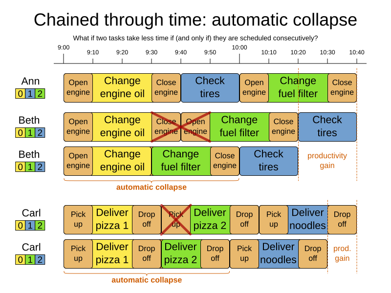
Implement the automatic collapse in the custom variable listener that calculates the start and end times of each task.
20.3.3.5. Chained through time: automatic delay until last
Some tasks require more than one person to execute. In such cases, both employees need to be there at the same time, before the work can start.
For example when assembling furniture, assembling a bed is a two-person job.
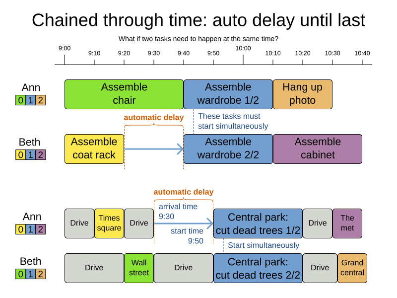
Implement the automatic delay in the custom variable listener that calculates the arrival, start and end times of each task. Separate the arrival time from the start time. Additionally, add loop detection to avoid an infinite loop:
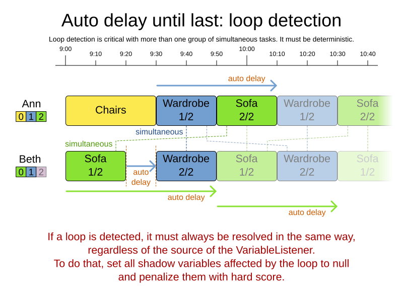
20.3.4. Time bucket pattern: assign to a capacitated bucket per time period
In this pattern, the time of each employee is divided into buckets. For example 1 bucket per week. Each bucket has a capacity, depending on the FTE (Full Time Equivalent), holidays and the approved vacation of the employee. For example, a bucket usually has 40 hours for a full time employee and 20 hours for a half time employee but only 8 hours on a specific week if the employee takes vacation the rest of that week.
Each task is assigned to a bucket, which determines the employee and the coarse-grained time period for working on it. The tasks within one bucket are not ordered: it’s up to the employee to decide the order. This gives the employee more autonomy, but makes it harder to do certain optimization, such as minimize travel time between task locations.
20.4. Cloud architecture patterns
There are two common usage patterns of OptaPlanner in the cloud:
-
Batch planning: Typically runs at night for hours to solve each tenant’s dataset and deliver each schedule for the upcoming day(s) or week(s). Only the final best solution is sent back to the client. This is a good fit for a serverless cloud architecture.
-
Real-time planning: Typically runs during the day, to handle unexpected problem changes as they occur in real-time and sends best solutions as they are discovered to the client.
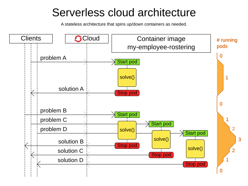
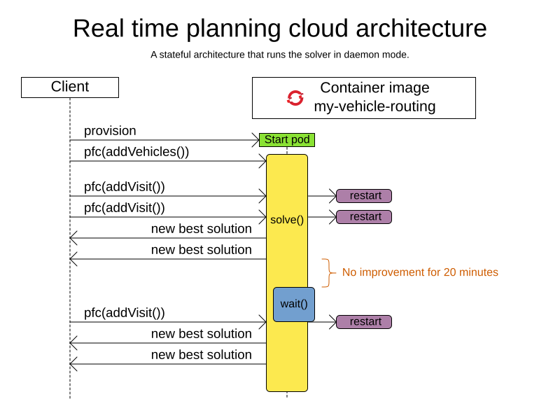
21. Development
21.1. Methodology overview
The diagram below explains the overall structure of the OptaPlanner source code:
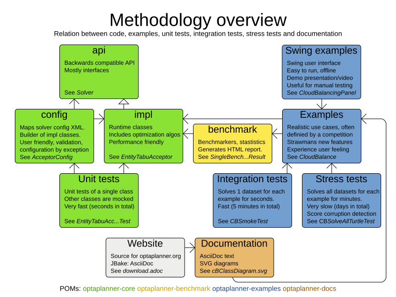
In the diagram above, it’s important to understand the clear separation between the configuration and runtime classes.
The development philosophy includes:
-
Reuse: The examples are reused as integration tests, stress tests and demos.
-
Consistent terminology: Each example has a class
App(executable class) andPanel(swing UI). -
Consistent structure: Each example has the same packages:
domain,persistence,app,solverandswingui. -
Real world usefulness: Every feature is used in an example. Most examples are real world use cases with real world constraints, often with real world data.
-
Automated testing: There are unit tests, integration tests, performance regressions tests and stress tests. The test coverage is high.
-
Fail fast with an understandable error message: Invalid states are checked as early as possible.
21.2. Development guidelines
21.2.1. Fail fast
There are several levels of fail fast, from better to worse:
-
Fail Fast at compile time. For example: Don’t accept an
Objectas a parameter if it needs to be aStringor anInteger. -
Fail Fast at startup time. For example: if the configuration parameter needs to be a positive
intand it’s negative, fail fast -
Fail Fast at runtime. For example: if the request needs to contain a double between
0.0and1.0and it’s bigger than1.0, fail fast. -
Fail Fast at runtime in assertion mode if the detection performance cost is high. For example: If, after every low level iteration, the variable A needs to be equal to the square root of B, check it if and only if an assert flag is set to true (usually controlled by the EnvironmentMode).
21.2.2. Exception messages
-
The
Exceptionmessage must include the name and state of each relevant variable. For example:if (fooSize < 0) { throw new IllegalArgumentException("The fooSize (" + fooSize + ") of bar (" + this + ") must be positive."); }Notice that the output clearly explains what’s wrong:
Exception in thread "main" java.lang.IllegalArgumentException: The fooSize (-5) of bar (myBar) must be positive. at ... -
Whenever possible, the
Exceptionmessage must include context. -
Whenever the fix is not obvious, the
Exceptionmessage should include advice. Advice normally starts with the word maybe on a new line:Exception in thread "main" java.lang.IllegalStateException: The valueRangeDescriptor (fooRange) is nullable, but not countable (false). Maybe the member (getFooRange) should return CountableValueRange. at ...The word maybe is to indicate that the advice is not guaranteed to be right in all cases.
21.2.3. Generics
-
The
@PlanningSolutionclass is often passed as a generic type parameter to subsystems. -
The
@PlanningEntityclass(es) are rarely passed as a generic type parameter because there could be multiple planning entities.
21.2.4. Lifecycle
One of the biggest challenges in multi-algorithm implementations (such as OptaPlanner) is the lifecycle management of internal subsystems. These guidelines avoid lifecycle complexity:
-
The subsystems are called in the same order in
*Started()and*Endedmethods.-
This avoids cyclic subsystem dependencies.
-
-
The
*Scopeclass’s fields are filled in piecemeal by the subsystems as the algorithms discover more information about its current scope subject.-
Therefore, a
*Scopehas mutable fields. It’s not anEvent. -
A subsystem can only depend on scope information provided by an earlier subsystem.
-
-
Global variables are sorted:
-
First by volatility
-
Then by initialization time
-
22. Release Notes
This chapter lists new and noteworthy updates in OptaPlanner releases. OptaPlanner follows a 3-week release cycle. Bug fixes and minor improvements are generally not announced, which is why some of the minor releases are not mentioned here.
For a step-by-step migration guide, see our upgrade recipe. We even provide a migration tool to make many of these changes automatically.
For release notes on OptaPlanner 7.x and older, please visit Release Notes on optaplanner.org.
22.1. OptaPlanner 8.x Release Notes
22.1.1. OptaPlanner 8.37.0.Final
22.1.1.1. PlanningListVariable supports nearby selection
Nearby selection is now available for planning domains using a planning list variable.
22.1.1.2. AbstractScoreHibernateType and its subtypes become deprecated
The AbstractScoreHibernateType as well as all its subtypes have been deprecated. The parallel OptaPlanner 9
releases are going to introduce Hibernate 6, which unfortunately breaks backward compatibility
of the CompositeUserType that the AbstractScoreHibernateType depends on.
The AbstractScoreHibernateType and its subtypes remain available in the OptaPlanner 8 releases to provide
integration with Hibernate 5 but have been removed from the equivalent OptaPlanner 9.x release.
To integrate the PlanningScore of your choice with Hibernate 6, either use the score converters available in the
org.optaplanner.persistence.jpa.api.score.buildin package or implement the CompositeUserType yourself.
22.1.2. OptaPlanner 8.36.0.Final
22.1.2.1. OptaWeb Vehicle Routing demo application abandoned
The codebase for OptaWeb Vehicle Routing demo application has been frozen and will no longer receive any updates.
We encourage users to check out the OptaPlanner Vehicle Routing Quickstart for a simple and straight-forward way of integrating OptaPlanner in your application.
22.1.3. OptaPlanner 8.35.0.Final
22.1.3.1. PlanningListVariable gets support for K-Opt Moves
A new move selector for list variables, KOptListMoveSelector, has been added.
The KOptListMoveSelector selects a single entity, removes k edges from its route, and add k new edges from the removed edges' endpoints.
The KOptListMoveSelector can help the solver escape local optima in vehicle routing problems.
Configuration options are available in the documentation.
22.1.3.2. SolutionManager gets support for updating shadow variables
SolutionManager (formerly ScoreManager) methods such as explain(solution) and update(solution) received a new overload with an extra argument, SolutionUpdatePolicy.
This has often been requested by users who load their solutions from persistent storage (such as a relational database), where these solutions do not include the information carried by shadow variables or even the score.
By calling these new overloads and picking the right policy,
OptaPlanner will automatically compute values for all the shadow variables in the given solution
and/or recalculate the score.
Similarly, ProblemChangeDirector received a new method called `updateShadowVariables(), so that you can update shadow variables on demand in real-time planning.
22.1.4. OptaPlanner 8.34.0.Final
22.1.4.1. Performance improvements in pillar moves and nearby selection
OptaPlanner can now auto-detect situations where multiple pillar move selectors can share a pre-computed pillar cache and reuse it instead of recomputing it for each move selector.
Users who combine different pillar moves (such as PillarChangeMove and PillarSwapMove) should see significant benefits.
The same applies to users of nearby selection. OptaPlanner can now auto-detect situations where a pre-computed distance matrix can be shared between multiple move selectors, saving a considerable amount of memory and CPU processing time.
As a consequence, implementations of the following interfaces are expected to be stateless:
-
org.optaplanner.core.impl.heuristic.selector.common.nearby.NearbyDistanceMeter -
org.optaplanner.core.impl.heuristic.selector.common.decorator.SelectionFilter -
org.optaplanner.core.impl.heuristic.selector.common.decorator.SelectionProbabilityWeightFactory -
org.optaplanner.core.impl.heuristic.selector.common.decorator.SelectionSorter -
org.optaplanner.core.impl.heuristic.selector.common.decorator.SelectionSorterWeightFactory
In general, if solver configuration asks the user to implement an interface, the expectation is that the implementation will be stateless or at the very least not try to include external state. With the aforementioned performance improvements, failing to follow this requirement will result in subtle bugs and score corruption as the solver will now reuse these instances as it sees fit.
22.1.4.2. OptaPlanner configuration becomes even more fluent
Various configuration classes, such as EntitySelectorConfig and ValueSelectorConfig,
received new builder methods which make it easier than ever
to replace XML-based solver config with fluent Java code.
22.1.5. OptaPlanner 8.33.0.Final
22.1.5.1. Value range auto-detection
In most cases, links between planning variables and value ranges can now be auto-detected.
Therefore, @ValueRangeProvider no longer needs to provide an id property.
Likewise, planning variables no longer need to reference value range providers via valueRangeProviderRefs property.
No code changes or configuration changes are required. Users who prefer clarity over brevity may continue to explicitly reference their value range providers.
22.1.6. OptaPlanner 8.32.0.Final
22.1.6.1. XStream support deprecated
Given that XStream has multiple CVEs against it and no recent releases,
we have decided to deprecate OptaPlanner’s support for serializing into XML using XStream.
To continue serializing into XML, please switch to the optaplanner-persistence-jaxb module.
All classes in the optaplanner-persistence-xstream, as well as the module itself, are now deprecated and will be removed in a future major version of OptaPlanner.
All examples in the optaplanner-examples module have been refactored to JSON using the optaplanner-persistance-jackson module.
Quickstarts were not affected by these changes, as they already were serializing into JSON.
22.1.7. OptaPlanner 8.31.0.Final
22.1.7.1. Several OptaPlanner examples removed from the distribution
In an ongoing effort to clean up code and reduce technical debt, the following examples were removed the optaplanner-examples module:
-
Batch Scheduling,
-
Cheap Time,
-
Coach Shuttle Gathering,
-
Investment
-
and Rock Tour.
We believe these examples were rarely used if ever, and they did not showcase any unique feature of OptaPlanner that would not be showcased already in any of the 16 remaining examples and many quickstarts.
No OptaPlanner feature was removed or deprecated in the process.
22.1.7.2. Multiple entity classes with chained planning variables
Fixed a bug that prevented using two or more chained planning variables, each defined on a different planning entity class.
22.1.8. OptaPlanner 8.30.0.Final
22.1.8.1. OptaPlanner operator (experimental) is available in the distribution
While the OptaPlanner operator remains experimental, it has now become a part of the OptaPlanner distribution.
If you want to learn more about the operator, follow the Kubernetes demo.
22.1.9. OptaPlanner 8.29.0.Final
22.1.9.1. Custom justifications and indictments in Constraint Streams
With a new Constraint Streams API, it is now easy to define custom constraint justifications and indictments in your constraints:
protected Constraint vehicleCapacity(ConstraintFactory factory) {
return factory.forEach(Customer.class)
.filter(customer -> customer.getVehicle() != null)
.groupBy(Customer::getVehicle, sum(Customer::getDemand))
.filter((vehicle, demand) -> demand > vehicle.getCapacity())
.penalizeLong(HardSoftLongScore.ONE_HARD,
(vehicle, demand) -> demand - vehicle.getCapacity())
.justifyWith((vehicle, demand, score) ->
new VehicleDemandOveruse(vehicle, demand, score))
.indictWith((vehicle, demand) -> List.of(vehicle))
.asConstraint("vehicleCapacity");
}Note the new methods: justifyWith(…) and indictWith(…). To find out more, see customizing justifications and indictments.
22.1.9.2. Compatible with JDK 19
OpenJDK 19 was recently released and OptaPlanner is fully compatible with it.
We always test our releases against the long-term supported versions of the JDK, currently 11 and 17, as well as against the latest release. We encourage you to upgrade your JDK regularly to benefit from the enhancements that come with the new releases.
22.1.9.3. New @ShadowVariable and @PiggybackShadowVariable annotations replace the @CustomShadowVariable
@ShadowVariable annotation is repeatable and allows to specify 1 listener per source variable.
@PiggybackShadowVariable is a specialized annotation to mark shadow variables that are updated by another shadow variable’s listener.
The @CustomShadowVariable has been deprecated.
Read more about custom shadow variables in the documentation.
22.1.9.4. Planning list variable
OptaPlanner now adds a limited support for planning list variables that can hold multiple planning values. The planning list variable provides an alternative approach to modeling planning problems that were previously modeled using the chained planning variable.
Both the planning list variable and the chained planning variable should be used with problems where the goal is to distribute a number of workload elements among limited resources in a specific order. For example, in vehicle routing, vehicles represent the limited resource and customers represent the workload elements.
The chained planning variable defines a recursive data structure, in which customers form chains ending with vehicles.
On the other hand, the planning list variable allows for a more intuitive model where each vehicle holds a list of customers it goes to.
It is defined using the new @PlaningListVariable annotation.
| The planning list variable is a new feature and lacks some advanced features, that are available with the chained planning variable. |
22.1.10. OptaPlanner 8.27.0.Final
22.1.10.1. Bavet is feature complete
The alternative constraint streams implementation Bavet is feature complete. You can now use it as an alternative to Drools (which is still the default).
Bavet will not be supported in Red Hat’s support offering. Drools intends to catch up performance wise.
22.1.11. OptaPlanner 8.24.0.Final
22.1.11.1. OptaWeb Employee Rostering demo application abandoned
The codebase for OptaWeb Employee Rostering demo application has been frozen and will no longer receive any updates.
We encourage users to check out the OptaPlanner Employee Rostering Quickstart for a simple and straight-forward way of integrating OptaPlanner in your application.
22.1.12. OptaPlanner 8.23.0.Final
22.1.12.1. Score DRL deprecated in favor of Constraint Streams
Support for Score DRL has been deprecated and users are encouraged to migrate to Constraint Streams at their earliest convenience. Read the migration guide from score DRL to Constraint Streams. Score DRL is not going away in OptaPlanner 8.
22.1.13. OptaPlanner 8.20.0.Final
22.1.13.1. SolverManager.addProblemChange() now returns CompletableFuture<Void>
SolverManager.addProblemChange() returns CompletableFuture<Void>, which completes when a new best solution containing
the problem change has been passed to a user-defined Consumer.
22.1.14. OptaPlanner 8.17.0.Final
22.1.14.1. Real-time planning available on the SolverManager
The SolverManager now accepts problem changes via the addProblemChange() method,
allowing for real-time planning
without much boilerplate code.
22.1.14.2. Faster Solver creation
SolverFactory newly caches some internal data structures, leading to much faster Solver creation times.
This is beneficial if you instantiate multiple Solver instances in quick succession.
22.1.15. OptaPlanner 8.12.0.Final
22.1.15.1. Documentation website
The latest final OptaPlanner documentation is now available on a new documentation website built using Antora. The single-HTML and PDF documentation will continue to be published in the archive.
22.1.15.2. Monitoring Support
OptaPlanner now uses Micrometer to monitor key metrics such as active solver count, solve durations, and error count.
22.1.16. OptaPlanner 8.10.0.Final
22.1.16.1. Support for Quarkus 2.0
OptaPlanner is now fully compatible with the recently released Quarkus 2.0.
22.1.17. OptaPlanner 8.7.0.Final
22.1.17.1. OptaPlanner quickstarts repository
There is a new quarkus-call-center quickstart that shows real-time planning of incoming calls in a call center.
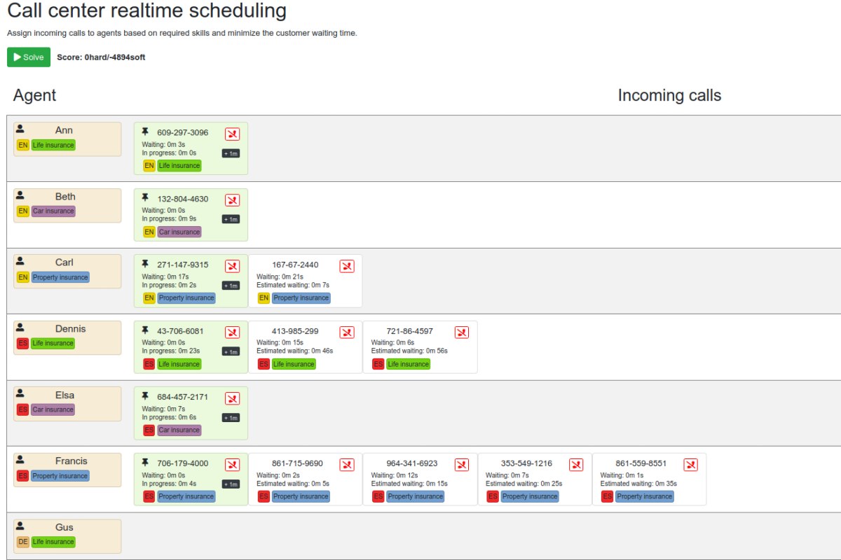
22.1.18. OptaPlanner 8.5.0.Final
22.1.18.1. Mapping in Constraint Streams
The Constraint Streams API received a major new functionality. You can now modify your streams using mapping functions.
22.1.18.2. Ready for OpenJDK 16
We have made some tweaks under the hood so that your experience with the recently released OpenJDK 16 continues to be smooth.
22.1.18.3. Inject and Autowire ConstraintVerifier in Quarkus and Spring Boot
You can now inject the Constraint Verifier in Quarkus and autowire the Constraint Verifier in Spring Boot, allowing you to test your constraint streams more easily.
22.1.18.4. OptaWebs on Quarkus
OptaWeb Vehicle Routing and OptaWeb Employee Rostering have been migrated from Spring Boot to Quarkus.
Other noteworthy changes done during the migration to Quarkus:
-
OptaWeb Vehicle Routing back end has a new RESTful API. Client-server communication, that was previously done using WebSockets, now uses a combination of REST calls and Server-Sent Events.
-
OptaWeb Employee Rostering now uses Constraint Streams instead of DRL for score calculation.
22.1.18.5. Faster domain accessors and cloning with Gizmo
We have added Gizmo generated domain accessors and solution cloners, which offer better performance than the reflection based domain accessors and solution cloners.
22.1.18.6. OptaPlanner quickstarts repository
There is a new activemq-quarkus-school-timetabling quickstart that shows how to integrate ActiveMQ with OptaPlanner to horizontally scale when solving multiple data sets.
22.1.19. OptaPlanner 8.3.0.Final
22.1.19.1. Major performance improvements for Constraint Streams
The default implementation of the Constraint Streams API has seen major performance improvements. Use cases with tri and quad streams may experience order of magnitude speedups. Use cases with grouping are likely to experience some speedups too, albeit comparatively smaller.
Kudos to the Drools team for helping make this possible!
22.1.19.2. Constraint Streams groupBy() overloads for multiple collectors
The Constraint Streams API has been extended to allow using more than 2 collectors in a single grouping. The following is now possible:
return constraintFactory.from(ProductPrice.class)
.groupBy(min(), max(), sum())
.penalize(..., SimpleScore.ONE, (minPrice, maxPrice, sumPrices) -> ...);22.1.20. OptaPlanner 8.0.0.Final
22.1.20.1. OptaPlanner quickstarts repository
The new OptaPlanner Quickstarts repository contains pretty web demos for several use cases. It also shows you how to integrate OptaPlanner with different technologies:
-
School timetabling: Assign lessons to timeslots and rooms to produce a better schedule for teachers and students.
This application connects to a relational database and exposes a REST API, rendered by a pretty JavaScript UI.
-
quarkus-school-timetabling: Java, Maven or Gradle, Quarkus, H2 -
spring-boot-school-timetabling: Java, Maven or Gradle, Spring Boot, H2 -
kotlin-quarkus-school-timetabling: Kotlin, Maven, Quarkus, H2
-
-
Facility location problem (FLP): Pick the best geographical locations for new stores, distribution centers, COVID-19 test centers or telco masts.
-
quarkus-facility-location: Java, Maven, Quarkus
-
-
Factorio layout: Assign machines to assembly line locations to design the best factory layout.
-
quarkus-factorio-layout: Java, Maven, Quarkus
-
-
Maintenance scheduling: Coming soon
22.1.20.2. Future Java compatibility
The OptaPlanner 8 API has been groomed to maximize compatibility with the latest OpenJDK and GraalVM releases and game-changing platforms such as Quarkus. Meanwhile, we still fully support OpenJDK 11 and platforms such as Spring Boot or plain Java.
For example, when running OptaPlanner in Java 11 or higher with a classpath,
OptaPlanner no longer triggers WARNING: An illegal reflective access operation has occurred for XStream.
22.1.20.3. Code completion for solverConfig.xml and benchmarkConfig.xml through XSD
To validate XML configuration during development, add the new XML Schema Definition (XSD) on the solver or benchmark configuration:
<?xml version="1.0" encoding="UTF-8"?>
<solver xmlns="https://www.optaplanner.org/xsd/solver" xmlns:xsi="http://www.w3.org/2001/XMLSchema-instance" xsi:schemaLocation="https://www.optaplanner.org/xsd/solver https://www.optaplanner.org/xsd/solver/solver.xsd">
...
</solver>This enables code completion for XML in most IDEs:
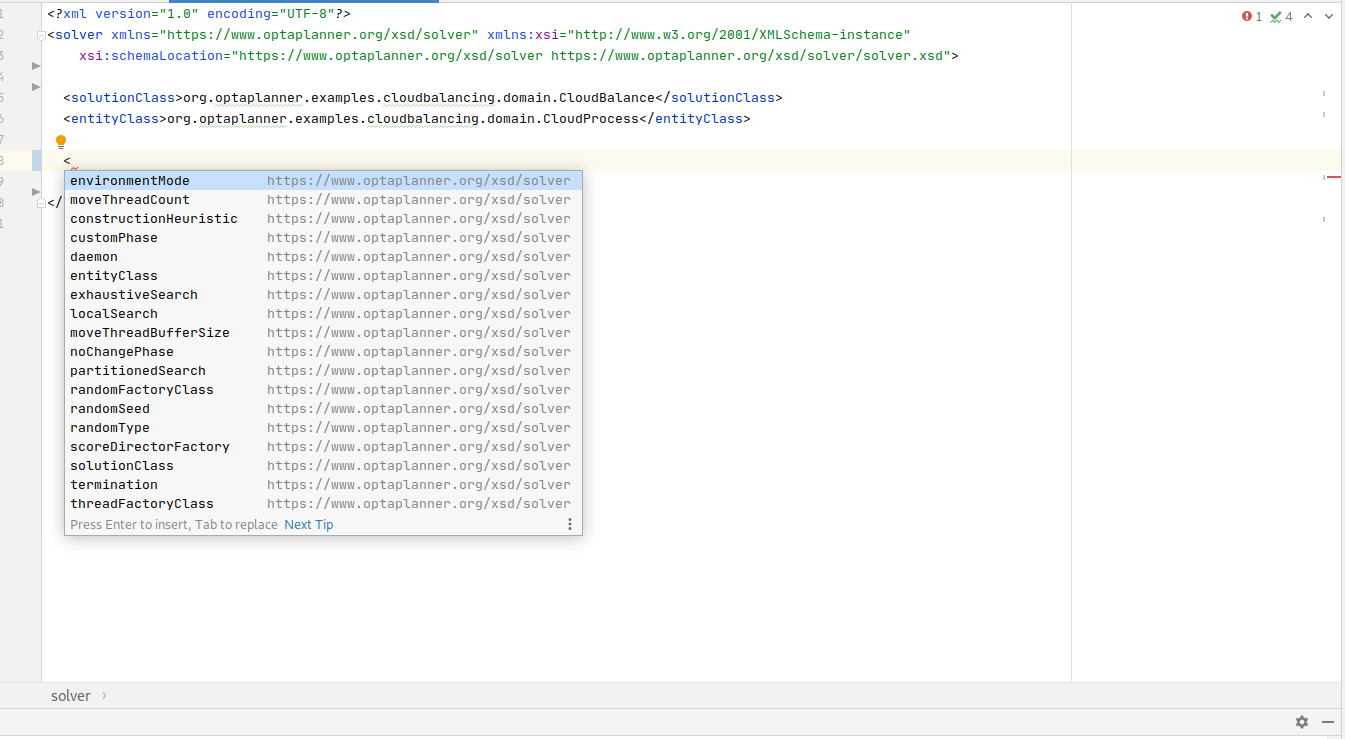
22.1.20.4. Improved Quarkus extension
The OptaPlanner Quarkus extension is now stable and displays no warnings when compiling Java to a native executable.
22.1.20.5. ScoreManager now supports score explanation
The ScoreManager can now also explain why a solution has a certain score:
ScoreManager<TimeTable, HardSoftScore> scoreManager = ScoreManager.create(solverFactory);
...
ScoreExplanation<TimeTable, HardSoftScore> scoreExplanation = scoreManager.explain(timeTable);
System.out.println(scoreExplanation.getSummary());
...Additionally, use scoreExplanation.getConstraintMatchTotalMap() and scoreExplanation.getIndictmentMap()
to extract the ConstraintMatchTotal<HardSoftScore> and Indictment<HardSoftScore> information without triggering a new score calculation.
22.1.20.6. Various improvements
-
The ConstraintStreams API is now richer, more stable with better error messages and faster.
-
The
SolverManagerAPI now supports to listen to both best solution events and the solving ended event. -
OptaPlanner no longer depends on Guava or Reflections.