Dealing with time and dates in planning problems may be problematic because it is dependent on the needs of your use case.
There are several representations of timestamps, dates, durations and periods in Java. Choose the right representation type for your use case:
java.util.Date(deprecated): a slow, error-prone way to represent timestamps. Do not use.javax.time.LocalDateTime,LocalDate,DayOfWeek,Duration,Period, ...: an accurate way to represent and calculate with timestamps, dates, ...Supports timezones and DST (Daylight Saving Time).
Requires Java 8 or higher.
On Java 7 use its backport called ThreeTen Backport instead.
On Java 6 or lower, use its predecessor called Joda Time instead.
intorlong: Caches a timestamp as a simplified number of coarse-grained time units (such as minutes) from the start of the global planning time window or the epoch.For example: a
LocalDateTimeof1-JAN 08:00:00becomes anintof400minutes. Similarly1-JAN 09:00:00becomes460minutes.It often represents an extra field in a class, alongside the
LocalDateTimefield from which it was calculated. TheLocalDateTimeis used for user visualization, but theintis used in the score constraints.It is faster in calculations, which is especially useful in the TimeGrain pattern.
Do not use if timezones or DST affect the score constraints.
There are also several designs for assigning a planning entity to a starting time (or date):
The starting time is fixed beforehand. It is not a planning variable (in such solver).
For example, in the hospital bed planning example, the arrival day of each patient is fixed beforehand.
This is common in multi stage planning, when the starting time has been decided already in an earlier planning stage.
The starting time is not fixed, it is a planning variable (genuine or shadow).
If all planning entities have the same duration, use the Timeslot pattern.
For example in course scheduling, all lectures take 1 hour. Therefore, each timeslot is 1 hour.
If the duration differs and time is rounded to a specifc time granularity (for example 5 minutes) use the TimeGrain pattern.
For example in meeting scheduling, all meetings start at 15 minute intervals. All meetings take 15, 30, 45, 60, 90 or 120 minutes.
If the duration differs and one task starts immediately after the previous task (assigned to the same executor) finishes, use the Chained Through Time pattern.
For example in time windowed vehicle routing, each vehicle departs immediately to the next customer when the delivery for the previous customer finishes.
Choose the right pattern depending on the use case:
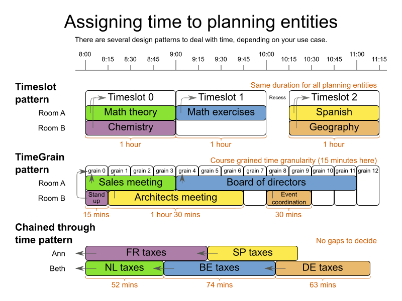
If all planning entities have the same duration (or can be inflated to the same duration), the Timeslot pattern is useful. The planning entities are assigned to a timeslot rather than time. For example in course timetabling, all lectures take 1 hour.
The timeslots can start at any time. For example, the timeslots start at 8:00, 9:00, 10:15 (after a 15-minute break), 11:15, ... They can even overlap, but that is unusual.
It is also usable if all planning entities can be inflated to the same duration. For example in exam timetabling, some exams take 90 minutes and others 120 minutes, but all timeslots are 120 minutes. When an exam of 90 minutes is assigned to a timeslot, for the remaining 30 minutes, its seats are occupied too and cannot be used by another exam.
Usually there is a second planning variable, for example the room. In course timetabling, two lectures are in conflict if they share the same room at the same timeslot. However, in exam timetabling, that is allowed, if there is enough seating capacity in the room (although mixed exam durations in the same room do inflict a soft score penalty).
Assigning humans to start a meeting at 4 seconds after 9 o'clock is pointless because most human activities have a time granularity of 5 minutes or 15 minutes. Therefore it is not necessary to allow a planning entity to be assigned subsecond, second or even 1 minute accuracy. The 5 minute or 15 minutes accuracy suffices. The TimeGrain pattern models such time accuracy by partitioning time as time grains. For example in meeting scheduling, all meetings start/end in hour, half hour, or 15-minute intervals before or after each hour, therefore the optimal settings for time grains is 15 minutes.
Each planning entity is assigned to a start time grain. The end time grain is calculated by adding the duration in grains to the starting time grain. Overlap of two entities is determined by comparing their start and end time grains.
This pattern also works well with a coarser time granularity (such as days, half days, hours, ...). With a finer time granularity (such as seconds, milliseconds, ...) and a long time window, the value range (and therefore the search space) can become too high, which reduces efficiency and scalability. However, such solution is not impossible, as shown in cheap time scheduling.
If a person or a machine continuously works on 1 task at a time in sequence, which means starting a task when the previous is finished (or with a deterministic delay), the Chained Through Time pattern is useful. For example, in the vehicle routing with time windows example, a vehicle drives from customer to customer (thus it handles one customer at a time).
In this pattern, the planning entities are chained. The anchor determines the starting time of its first planning entity. The second entity's starting time is calculated based on the starting time and duration of the first entity. For example, in task assignment, Beth (the anchor) starts working at 8:00, thus her first task starts at 8:00. It lasts 52 mins, therefore her second task starts at 8:52. The starting time of an entity is usually a shadow variable.
An anchor has only one chain. Although it is possible to split up the anchor into two separate anchors, for example split up Beth into Beth's left hand and Beth's right hand (because she can do two tasks at the same time), this model makes pooling resources difficult. Consequently, using this model in the exam scheduling example to allow two or more exams to use the same room at the same time is problematic.
Between planning entities, there are three ways to create gaps:
No gaps: This is common when the anchor is a machine. For example, a build server always starts the next job when the previous finishes, without a break.
Only deterministic gaps: This is common for humans. For example, any task that crosses the 10:00 barrier gets an extra 15 minutes duration so the human can take a break.
A deterministic gap can be subjected to complex business logic. For example in vehicle routing, a cross-continent truck driver needs to rest 15 minutes after 2 hours of driving (which may also occur during loading or unloading time at a customer location) and also needs to rest 10 hours after 14 hours of work.
Planning variable gaps: This is uncommon, because an extra planning variable (which impacts the search space) reduces efficiency and scalability.
For practical or organizational reasons (such as Conway's law), complex planning problems are often broken down in multiple stages. A typical example is train scheduling, where one department decides where and when a train will arrive or depart, and another departments assigns the operators to the actual train cars/locomotives.
Each stage has its own solver configuration (and therefore its own SolverFactory). Do not
confuse it with multi-phase solving which uses a one-solver configuration.
Similarly to Partitioned Search, multi-stage planning leads to suboptimal results. Nevertheless, it may be beneficial in order to simplify the maintenance, ownership, and help to start a project.